Recall that we want to prove
Proof
For the forward direction, we want to show that every \(\mathcal{V}\)-polyhedron is an \(\mathcal{H}\)-polyhedron. Given some \(\mathcal{V}\)-polyhedron \(P\). Let
A point in \(\operatorname{conv}(V)\) has the form \(t_1v_1+\cdots+t_nv_n\) where \(t_i \ge 0\) and \(t_1+\cdots+t_n=1.\). Similarly, a point in \(\operatorname{cone}(Y)\) has the form \(u_1y_1+\cdots+u_{n'}y_{n'}\) where \(u_j \ge 0.\). Therefore a point in \(\operatorname{conv}(V)+\operatorname{cone}(Y)\) has the form
where \(t_i\ge0, u_j\ge0\) and \(\sum_{i=1}^{n} t_i=1.\). If we form the matrices
and the coefficient vectors
then the expression above can be written compactly as
The condition \(\mathbf{1}t=1\) is simply \(t_1+\cdots+t_n=1,\) where \(\mathbf{1} = \begin{bmatrix} 1 & \cdots & 1 \end{bmatrix}.\) Hence
Next define
Rather than looking only at the points \(x\), we introduce the coefficient vectors \(t\) and \(u\) as additional variables. Thus every point \(x\) is lifted to the point \((x,t,u)\) in the higher-dimensional space \(\mathbb{R}^{d+n+n'}\). The advantage of introducing \(Q\) is that all of the defining conditions
are linear equations and inequalities. Therefore \(Q\) is naturally described as an intersection of finitely many affine hyperplanes and halfspaces, so \(Q\) is an \(\mathcal{H}\)-polyhedron. The original set \(\operatorname{conv}(V)+\operatorname{cone}(Y)\) can be recovered from \(Q\) by forgetting the variables \(t\) and \(u\) and keeping only the \(x\)-coordinates.
So now we know that \(Q\) is an \(\mathcal{H}\)-polyhedron but what we want is to show that the projection of \(Q\) gives us an \(\mathcal{H}\)-polyhedron which is the original set. In other words, we want to show that
where the projection is
Though in the textbook, instead of proving the projection theorem in full generality, they project along a coordinate axis and eliminate one variable. So suppose
and suppose that we want to eliminate the variable \(x_k\). The way to do this is using the Fourier-Motzkin Elimination method which goes like this: if we have a system of linear inequalities, isolate the variable we want to drop (\(x_k\)) and collect all the constraints where \(x_k\) is on the “greater side” and all the constraints where \(x_k\) is on the “less side”. The projection is then simply the system of inequalities that you get by pairing every single lower bound with every single uppoer bound. A small example is below
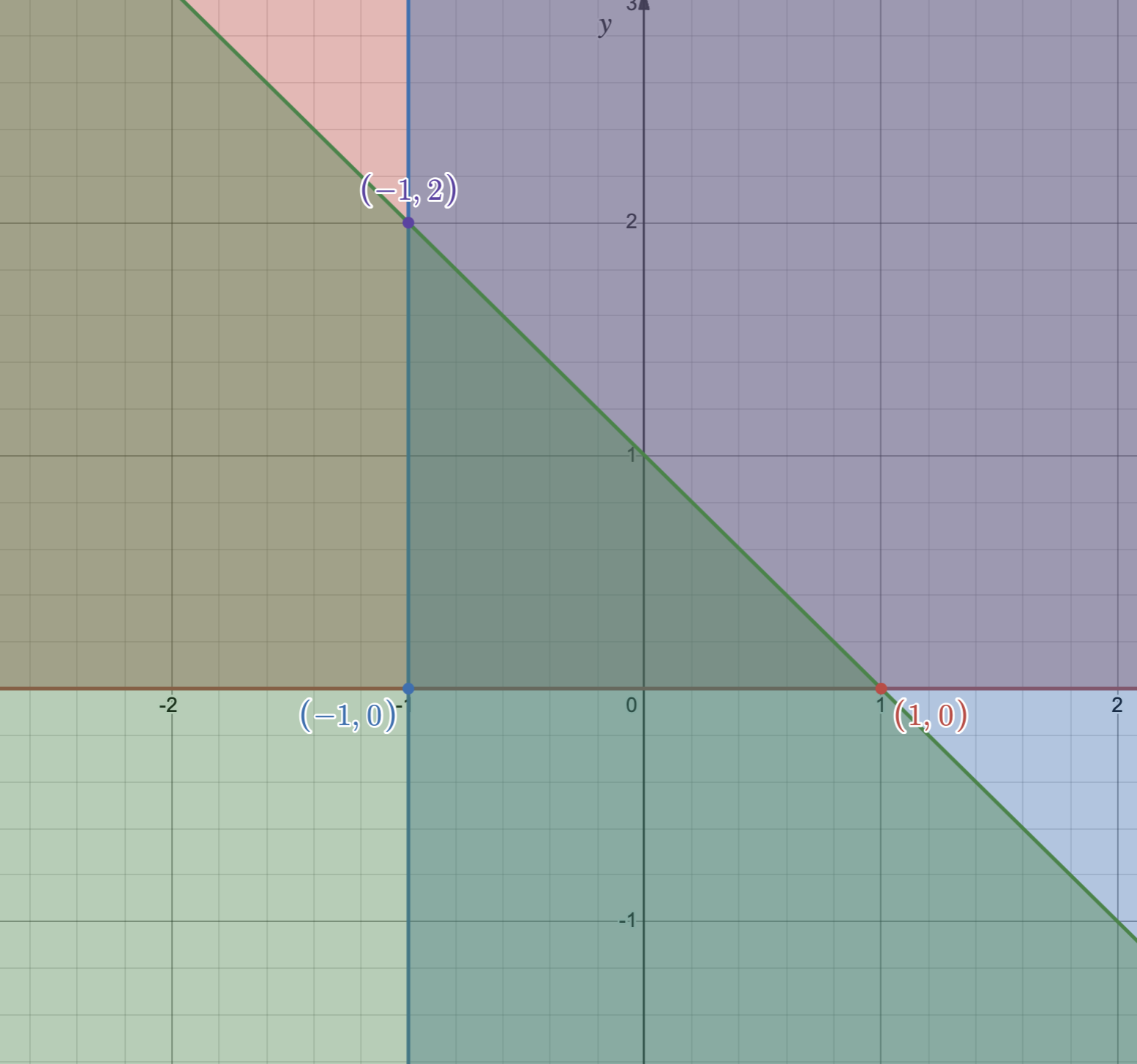
- \(x + y \le 1\)
- \(y \ge 0\)
- \(x \ge -1\)
- From (1), \(y \le 1 - x\) (Upper Bound)
- From (2) \(y \ge 0 \) (Lower Bound)
The textbook then defines
So given a point \(x\) in the polyhedron, we just subtract its \(k\)th component. So the \(k\)th component just becomes \(0\) while the remaining coordinates remain untouched. This is equivalent to
So it’s the other way around. A point \(x \in \mathbb{R}^d\) is in the set if its \(x_k\) component is zero and there exists some \(y \in \mathbb{R}\) such \(x + ye_k\) is a point in \(P\). Note that this projection is contained entirely in the hyperplane
Moreover, consider the set
unlike \(\operatorname{proj}_k(P)\) which drops a dimension. \(\operatorname{elim}_k(P)\) is still full dimensional. For the triangle example above, \(\operatorname{proj}_k(P)\) is the line segment where \(-1 \leq x \leq 1\) and \(y=0\). However, \(\operatorname{elim}_k(P)\) is the entire plane such that \(-1 \leq x \leq 1\). Moreover, observe that
This leads to the isomorphism
The reason why we want to work with \(\operatorname{elim}_k(P)\) is because we stay in the same dimension and avoid dropping a dimension every time we drop a coordinate.
So the goal or plan is take the original set and lift it to the set \(Q\). Now we apply Fourier-Motzkin Elimination described in the triangle example above to get \(elim_k(Q)\) which as we saw is an \(\mathcal{H}\)-polyhedron since it a set of linear inequalities. but as we saw above, \(elim_k(Q)\) is isomorphic to \(\operatorname{proj}_k(Q) \times \mathbb{R}\). Hence \(\operatorname{proj}_k(Q)\) is also an \(\mathcal{H}\)-polyhedron.
To describe Fourier-Motzkin Elimination for eliminating \(x_k\), we isolate the coordinate variable \(x_k\). Let \(a_i\) denote the \(i\)-th row of the matrix \(A\). The dot product \(a_i x\) expands to include the \(k\)-th coordinate explicitly:
\(a_i x = a_{i1}x_1 + \dots + a_{ik}x_k + \dots + a_{id}x_d\)
The expression \(a_i x - a_{ik}x_k\) represents a linear combination of all variables except \(x_k\). This allows us to isolate \(x_k\) for any pair of constraints.
First, we isolate \(x_k\) into Upper and Lower Bounds. We choose an index \(i\) where \(x_k\) acts as an upper bound (\(a_{ik} > 0\)) and an index \(j\) where \(x_k\) acts as a lower bound (\(a_{jk} < 0\)).
- Upper Bound (\(a_{ik} > 0\)):
$$ \begin{align*} a_i x \le z_i &\implies a_{ik}x_k + (a_i x - a_{ik}x_k) \le z_i \\ &\implies a_{ik}x_k \le a_{ik}x_k - a_i x + z_i \end{align*} $$
- Lower Bound (\(a_{jk} < 0\)): Since \(a_{jk}\) is negative, the coefficient \(-a_{jk}\) is strictly positive. We rewrite the \(j\)-th constraint to isolate \(x_k\) on the greater-than side:
$$ \begin{align*} a_j x \le z_j &\implies a_{jk}x_k + (a_j x - a_{jk}x_k) \le z_j \\ &\implies -z_j + (a_j x - a_{jk}x_k) \le -a_{jk}x_k \\ &\implies (-a_{jk})x_k \ge -a_{jk}x_k + a_j x - z_j \end{align*} $$
Next, to eliminate \(x_k\), the leading coefficients on \(x_k\) must match. We multiply the upper bound inequality by the positive scalar \((-a_{jk})\) and the lower bound inequality by the positive scalar \(a_{ik}\):
A valid coordinate \(x_k\) exists if and only if the scaled lower bound is less than or equal to the scaled upper bound:
Expanding both sides yields:
Notice that the \(-a_{ik}a_{jk}x_k\) terms appear identically on both sides and cancel completely, removing \(x_k\) from the system to get
Gathering all terms involving the remaining vector \(x\) to the left side and the constants to the right side gives the final eliminated linear inequality:
Because \(\left(a_{ik}a_j + (-a_{jk})a_i\right)\) is simply a new constant row vector \(A'\) and \(a_{ik}z_j + (-a_{jk})z_i\) is a new scalar constant \(z'\), this expression simplifies to:
Pairing every finite upper bound with every finite lower bound generates a new, finite system of linear inequalities. Thus, \(\operatorname{elim}_k(P)\) remains an \(\mathcal{H}\)-polyhedron which is what we wanted to show.