These notes are taken from watching the video in the reference. Suppose we want to graph the function of the form,

$$ \begin{align*} f(x) = a^x \end{align*} $$

First, if $a < 0$, then we’ll run into complex numbers and other issues so typically the exponential function is defined for any base that is greater than zero. So Suppose $a > 0$. We will still see that we have three cases:

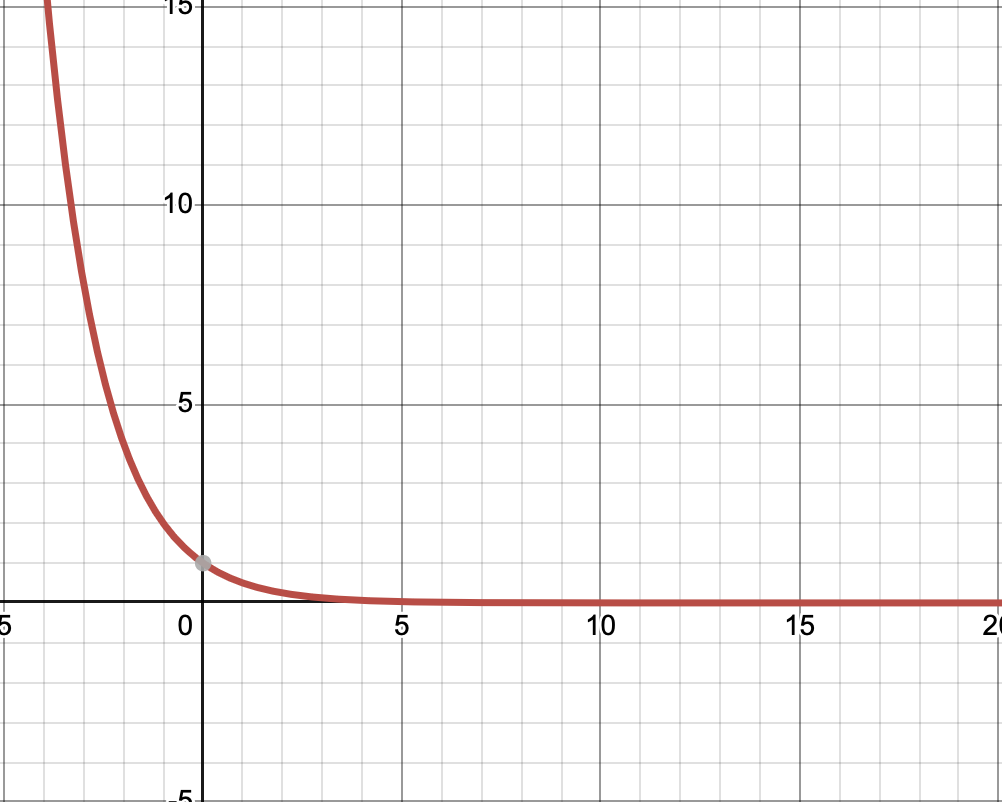
When $$a < 1$$, we'll see something like this: (this is the function $$0.5^x$$). As $$x$$ gets larger, $$y$$ will approach $$0$$. We can see this because $$f(1) = 1/2$$, $$f(2) = 1/4, f(3) = 1/8$$ and so on.
When $$a = 1$$, we'll see just the line $$y = 1$$. $$1^x$$ is 1 no matter what $$x$$ is! so not really interesting.
When $$a > 1$$, for example when $$f(x) = 2^x$$, then as the exponent gets bigger, we'll approach infinity. $$f(1) = 2, f(2) = 4, f(3) = 0$$ and so on.

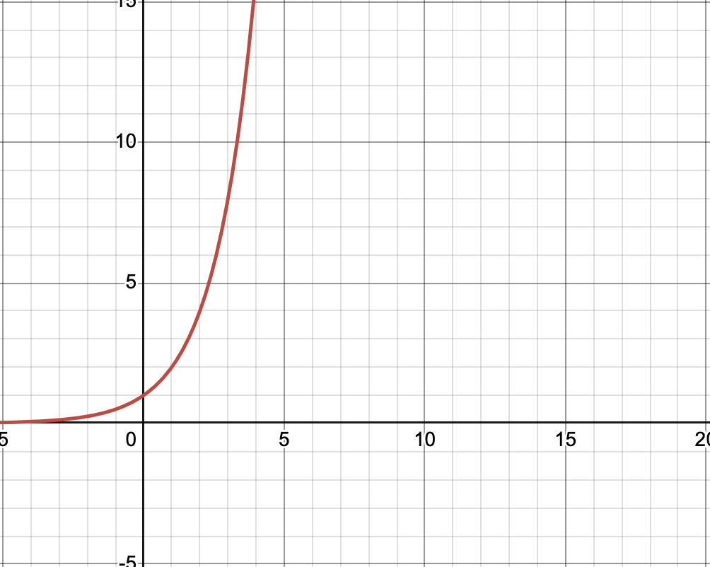
The trick to graphing these functions to always remember that we always have the points $(0,1)$ and $(1,a)$ plotted on our graph! so always evaluate the inputs $0$ and $1$.

The Domain and Range

It’s important to know the domain and range to help see what the functions would look like. The domain here is any real number so $(-\infty, \infty)$. What about the range? We can never reach any number that is zero or below so the range can be written as $(0, \infty)$. This also means that $y=0$ is a horizontal asymptote.

Vertical Asymptotes

The domain is all the real numbers so we don’t have any domain issues and so we won’t have any vertical asymptotes.

Horizontal Asymptotes

so I know intuitively that for $a^x$ for example, the graph never reaches 0 no matter what $x$ values we plug in. This means that $y=0$ is a horizontal asymptote. I’ve also seen tutorials define the asymptote of exponential functions of the form $f(x)=ca^{x+b}+d$ to be $d$. Either way? it’s kind of clear? or maybe now?

$$e^x$$

$e^x$ comes up frequently but is there anything special about graphing it? not really. It is very similar to the above.

Vertical Shift

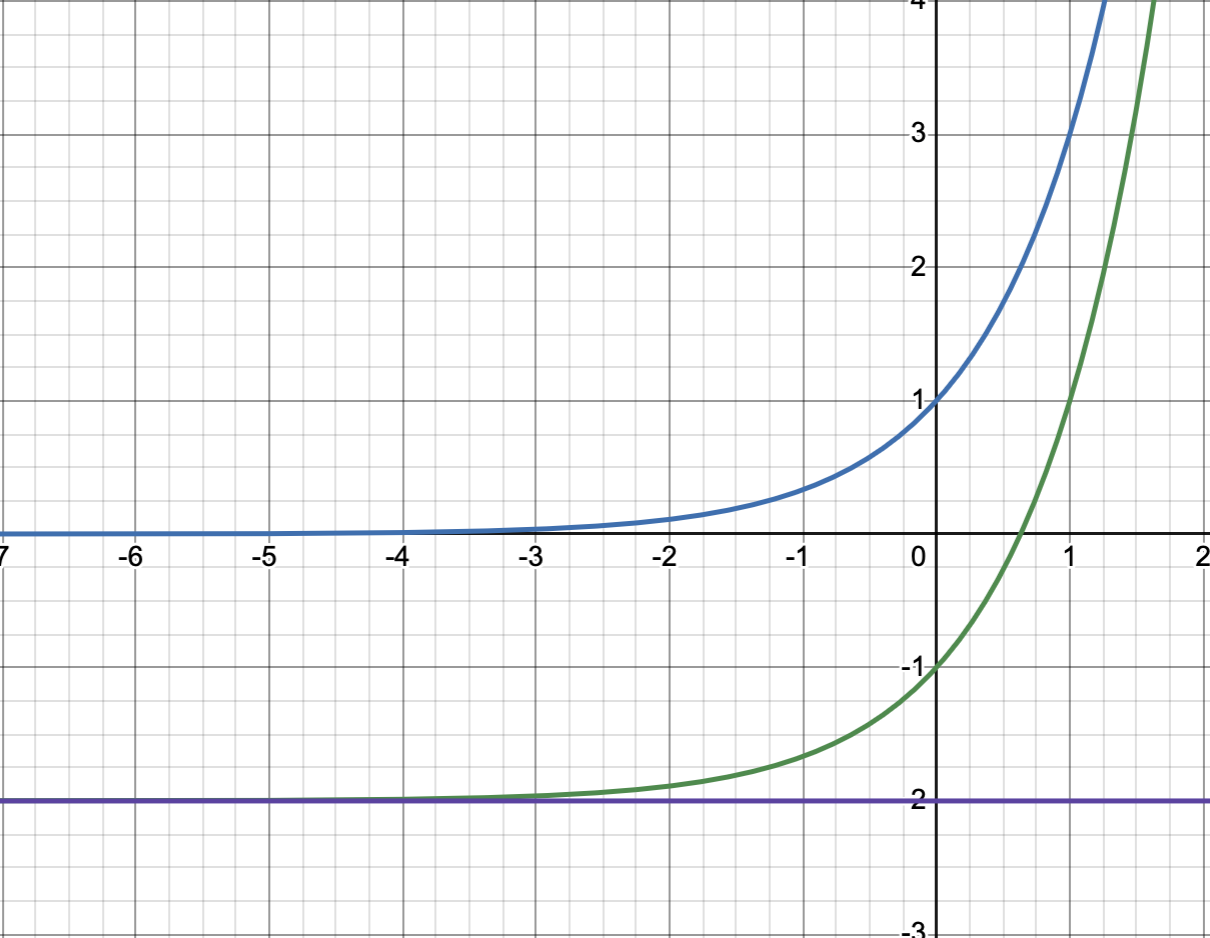
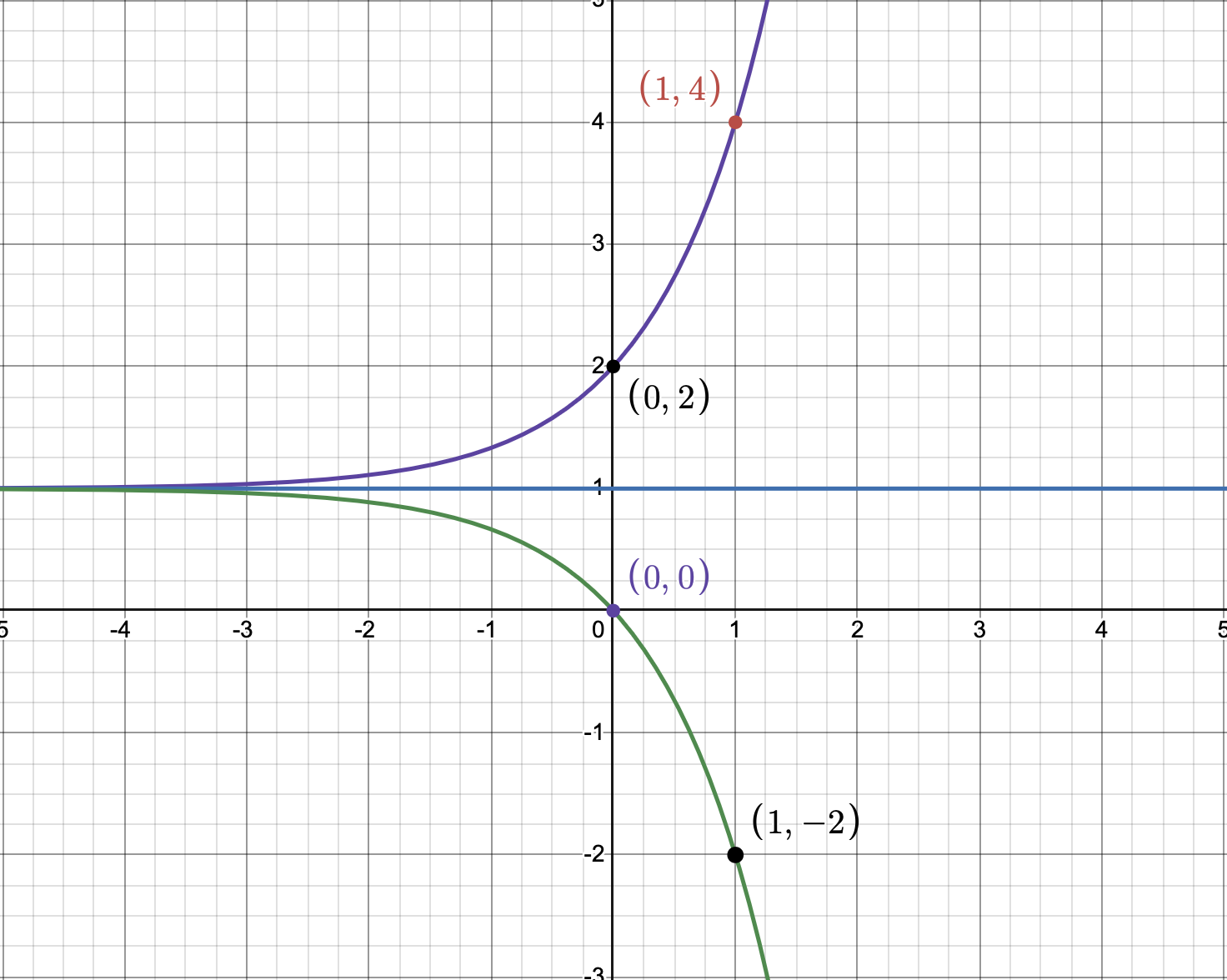
What happens if we’re about to graph a function like $3^x - 2$. Notice here that we have a $-2$. This is a vertical shift that will shift be the whole graph of the function down two units (green curve moved down 2 units from the original blue curve). Note that the horizontal asymptote is also going to shift to -2.

Horizontal Shift

A horizontal shift example is the following:

$$ \begin{align*} f(x) = 2^{x+2}. \end{align*} $$

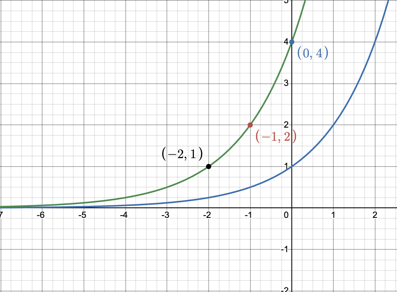
We know originally we had $2^x$ along with a horizontal asymptote at $y=0$ and the points $(0,1)$ and $(1,2)$. What’s going to happen now? The whole graph is going to shift 2 points to the left (opposite of the sign in the exponent). This means that the x coordinates of the all the points we plotted for the original graph will now decrease by two. So $(0,1)$ will be $()-2,1)$. Similarly, $(1,2)$ will now be $(-1,2)$. One more thing that we usually plot is the y-intercept. To find it, we just evaluate $f(0) = 2^{0+2} = 4$. The horizontal asymptote is unaffected here.

Reflection Around the Horizontal Asymptote

Suppose we’re graphing the following function:

$$ \begin{align*} f(x) = -3^x + 1. \end{align*} $$

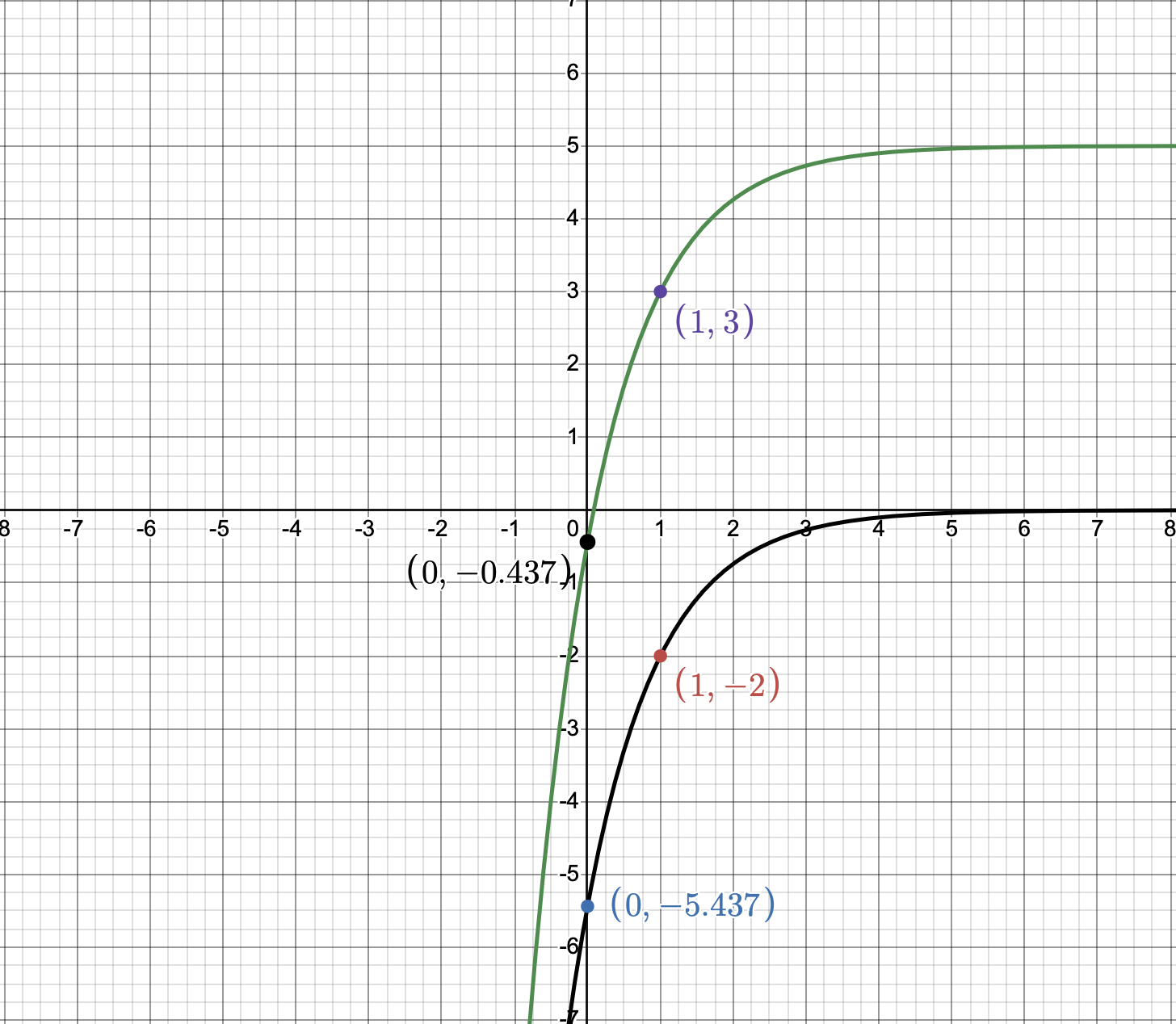
We can see here that we have a negative sign in front of the exponential. $(- (3^x))$. This negative sign will reflect the whole curve around its horizontal asymptote which is $y=1$ in this example. To graph this function, let’s start by graphing the original function $3^x$ with the known two points $(0,1)$ and $(1,3)$ as well as the horizontal asymptote at $y=0$.

Next,

We have a vertical shift (+1) and so the horizontal asymptote will move up by one point be $$y=1$$. So the new points will be $$(0,2)$$ and $$(1,4)$$. The black curve ($$3^x$$) shifts up to become the purple curve ($$3^x+1$$).
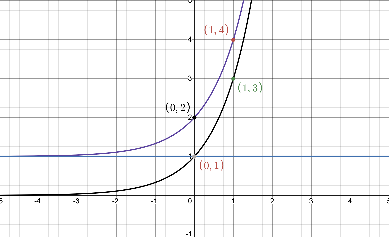
The negative sign infront reflects the curve around the horizontal asymptote $$y=1$$. For this step it might also be easier to also evaluate the known points keeping in mind that we expect to see a reflection so $$f(0) = -(3^0)+1=0$$ and $$f(1) = -(3^1)+1=-2$$.

More Examples

Suppose we’re graphing the following function:

$$ \begin{align*} f(x) = 5 - 2e^{-x+1}. \end{align*} $$

We have a lot going on here. Let’s re-arrange so that:

$$ \begin{align*} f(x) = - 2e^{-(x-1)} + 5. \end{align*} $$

Before diving in, let’s graph the $e^x$ so we can have something to compare against.

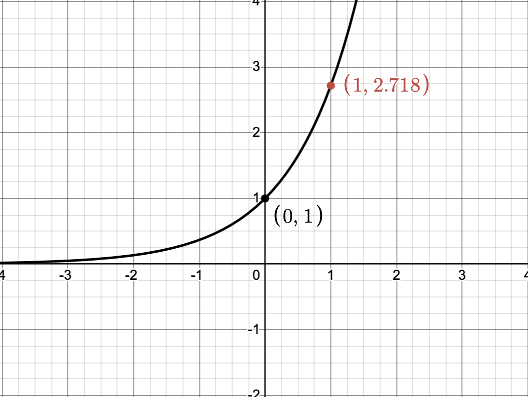
So this is $e^x$ along with the points $(0,1)$ and $(1,e)$. Now, let’s dive into the transformations:

If we look at the exponent and inside the parenthesis, we see that we have a -1. This means that it's a shift to the right by 1. This also means that our points' x-coordinates will shift by 1 and so $$(0,1)$$ and $$(1,e)$$ will now be $$(1,1)$$ and $$(2,e)$$.

But what about the negative sign outside the parenthesis in the exponent? This negative sign will reflect the graph around the y-axis. But it's tricker here because we moved the points 1 point to the right! so what we want to reflect this graph around $$x=1$$ instead.
The red curve above is the graph of $$e^{-(x-1)}$$.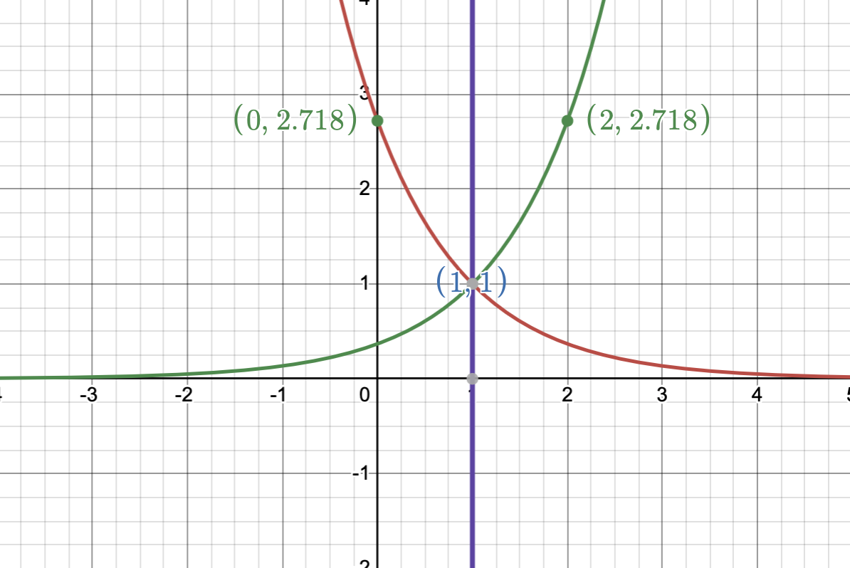
Next we have the "2" factor at the beginning will just stretch the graph vertically by 2. There is also a negative sign. This negative sign will cause the curve to get reflected around the horizontal asymptote this time.

Finally, the vertical shift is 5 so the horizontal asymptote moves to $$y=5$$ and the y-coordinate of all the points will be increased by 5.

References: