Note

These are my rough notes based on attending CS148. They might contain errors so proceed with caution!

Overview

In the global illumination lecture we talked about bidirectional ray tracing. It combined both photon tracing (forward) and ray tracking (backward). We said that we will emit photons from the light, bathe these objects in light in order to create a light map. We will then use this light map when we ray trace the scene to estimate the indirect light instead of just relying on the ambient term.

We then discussed the fact that the lighting equation can be used to described any point in any direction and we discovered that it is an implicit equation that can fit into a well known category (Fredholm Integral Equation) and this allowed us to discretize it which wasn’t tractable so we had to rely on radiosity and albedo from computer vision which led to a more tractable form. But today we will instead use Monte Carlo.

Photon Maps

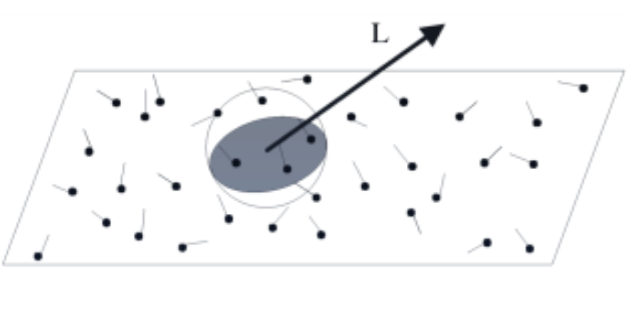
To create a photon map, we’ll emit photons from light sources and bounce around the scene. In the figure above, we have a number photons photons where each photon is storing the incoming light direction with the strength just like regular lights. If we want to know the pixel color at a point for example (the $L$ viewing direction in the picture), we’ll sum over the light from all the photons nearby and sum over all of these just like regular lights. Note that we’ll still be doing the important sampling and handle direct light with shadow rays and sum this amount as well. We could use a photon map for all lighting but it will require a ton of photons so it’s easier to still do the direct lighting with shadow rays.

To create a light map, we will emit a photon like the figure until it intersects something. If we hit direct light, then we ignore it. If it’s not then we have two choices assuming it doesn’t get absorbed (see the two arrows in the figure). So now we need to decide if this photon will get absorbed. If it does, then it’s gone and we don’t care. If it bounces, then we’ll need to determine the probability of it being specul Screenshot 2023 10 28 At 10.07.45 AM ar vs diffuse. Roll some dice and decide! but it has to be one or the other.

Next, if this photon hits say a camera and bounces, then that’s two bounces! we’ll bounce it until hits an object and then store the value in the photon map. We’ll take the point of intersection, the incoming light direction and store both in the photon map. This photon might bounce again and if it hits another object, we’ll store that intersection along with the incoming light direction in the map again (another entry for the same photon). Notice here that one we choose diffuse, we are stuck here unlike if we get specular, then we’ll have two choices again.

Tractability

In the global illumination lecture, we discretized surfaces and hemisphere directions. too many chucks (curse of dimensionality).

Another way to solve this is using Monte Carlo integration. Instead of discretizing, we’ll functions that generate pseudo random sequences.

Monte Carlo Integration: No curse of dimensionality. Scales to higher dimensions. The purely diffuse lighting assumption is not needed.

Example of Monte Carlo Integration

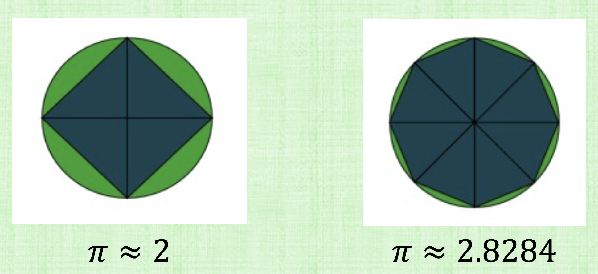
as opposed to Newton-Cote. Consider approximating $\pi$. You need a compass. Draw a circle of with radius of one unit distance. The area is $A=\pi r^2$ and therefore, the area is just $\pi$. So we just need to find the area of the circle. Integrate $f(x,y)=1$ over the unit circle to obtain $\int\int_A f(x,y)dA = \pi$.

For Newton-Cotes, we’ll inscribe triangles inside te circle. Find the sum of the area of the all the triangles.

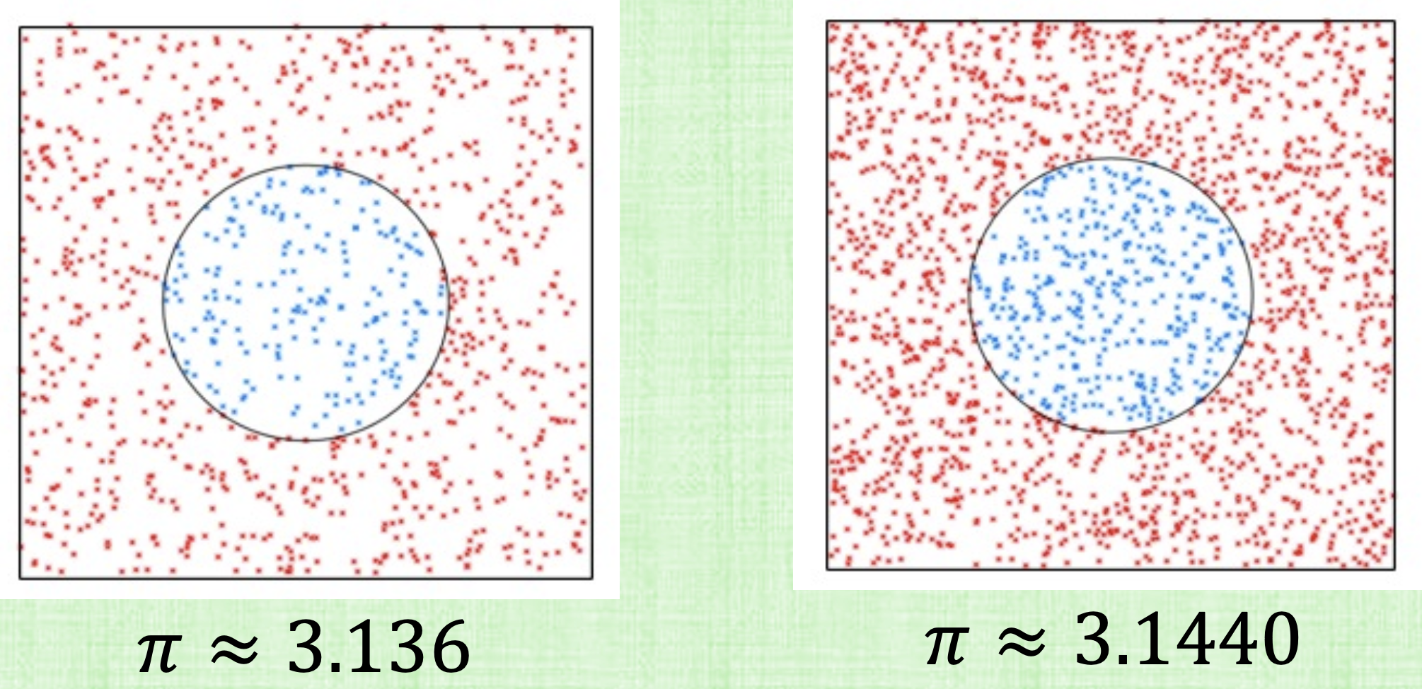
For Monte Carlo, construct a square with side length 4 containing the circle. Generate $N$ points in the square. Color the points inside the circle blue. Since $\frac{A_{circle}}{A_{box}} = \frac{pi}{16}$, then we can approximate $pi$ ~ 16 \frac{N_{blue}}{N_{blue}+N_{red}}$.

Monte Carlo Methods

Random (pseudo-random) numbers generate sample points that are multiplied by some element size (length, area, volume). Basically each point in enclosed in some sample area size are if we’re working in 2D. They might overlap but that’s find. The error decreases by $1/\sqrt{N}$ where $N$ is the number of samples. Monte Carlo is good for higher dimensions while Newton-Cote is much better in 1/2/3D.

1D example. Consider solving,

$$ \begin{align*} \int_a^b f(x)dx. \end{align*} $$

Generate $N$ random samples $X_i$ in the interval $[a, b]$. A Monte-Carlo estimate for the integral is

$$ \begin{align*} F_N &= \sum_{i=1}^N \frac{b-a}{N}f(X_i) \\ &= (b - a)\frac{\sum_{i=1}^N f(X_i)}{N} \end{align*} $$

This is a simple averaging of all the sample results.

Important Sampling

Sometimes we want to cheat with what samples we want to pick. If we have a function that is flat in some range and not flat in some other range, we’d want to pick samples from the non-flat range. For example, suppose $f(x)$ is only non-zero in $[a_1, b_1] \subset [a,b]$ so that $\int_a^b f(x)dx = \int_{a_1}^{b_1} f(x)dx$. In this case, if $X_i \notin [a_1, b_1]$ doesn’t contribute to the integral.

In general, the probability distribution $p(x)$ should prefer samples from areas with higher contribution to the integral (important sampling). Given a $p(x)$ with $\int_a^b p(x)dx = 1$, the Monte Carlo estimate is:

$$ \begin{align*} F_N &= \frac{1}{N} \sum_{i=1}^N \frac{1}{p(X_i)}f(X_i) \end{align*} $$

where $p(x)=1/(b-a)$ (uniform sampling). This reduces to

$$ \begin{align*} F_N &= (b -a) \frac{\sum_{i=1}^N f(X_i)}{N} \end{align*} $$

Photon Emission

Photon Strength: We’ll choose some number of photons and divide them amongst the lights (based on relative power). Photons all have the same power but brighter lights will just have more photons.

Photon Position: For point lights, all photons are emitted from a single point. For area lights, we’ll randomly select a point on the surface to emit the photon from. We’ll divide the rectangular light into a uniform 2D grid and emit a set of photons from each grid cell (randomly choosing the position within the cell).

Emission Direction: Randomly choose a direction on a sphere, a hemisphere or a subset of the sphere (for point lights). In some cases like the sun, a large number of photons would miss the scene entirely so ignore these photons (don’t emit them) and restrict the light to a sub-light and so on.

Light Map

We will have a different photon map for each color.
Use a ray tracer and once we intersect an object, then store the intersection point along with the incoming light direction (no need to store the strength if all photons have the same strength). just like what we said earlier. Make a copy of the photon’s data to store it in the light map.
To measure absorption, generate a random number between 0 and 1 and compare it to the probability of absorption. If absorbed, then the process stops for this photon. Otherwise, we continue to bounce.
To compute a bounce direction, we map BRDF directions into probabilities. For example a purely diffuse BRDF has equal probabilities for every hemisphere direction. We again generate a random number and use it to determine the bounce direction and then we’ll use a ray tracer to trace that path.
We will use a pre-determined maximum number of bounces before we terminate.
Typically photon maps are stored in an octree or kd-tree structure.

Separating Diffuse/Specular

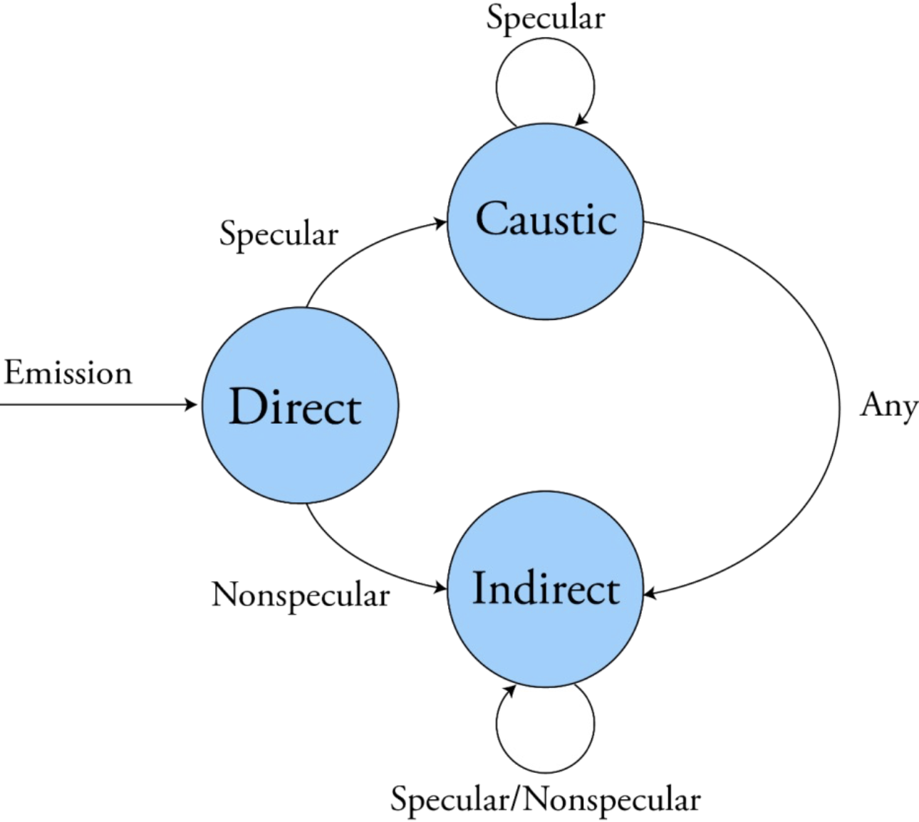
It’s more convenient to store diffuse and specular lighting separately. So when bouncing a photon, determine randomly if the photon will

get absorbed
will be diffuse bounced
will be specular bounced
We then determine the bounce direction randomly with the appropriate BRDF (diffuse/specular)
We will use two light maps (1) Caustic Maps: stores the photons that have had specular bounces only. (2) Indirect Lighting Map: store the photons that have had at least one diffuse bounce.

Gathering Radiance

Trace rays from the camera and intersect with objects and use shadow rays for direct lighting.
Estimate radiance contribution to the ray from caustics and indirect lighting using the respective light maps: use the N closest photons to the point of intersection (with the aid of the acceleration structure (octree or kdtree))

Color

3 photon maps one for each color. Objects of certain color better absorb photons of differing colors so this gives color bleeding and related effects.

References

Fundamentals of Computer Graphics, 4th Edition
CS148 Lectures