These are notes I took while watching the series The Essence of Linear Algebra by 3Blue1Brown.
Linear Transformations Recap
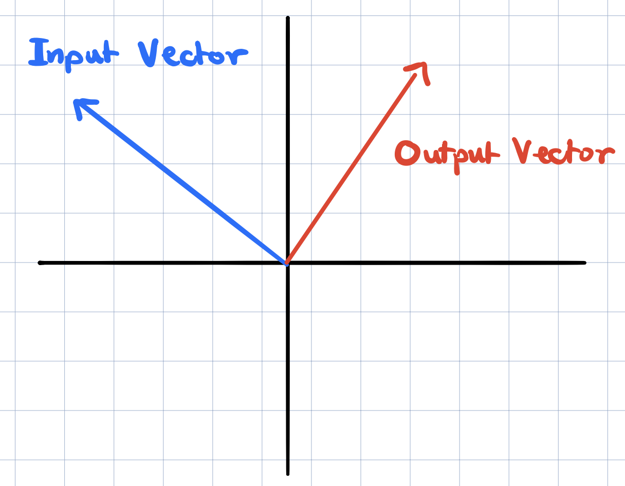
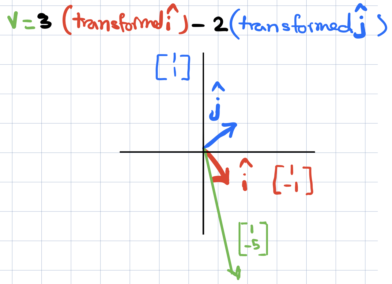
Linear transformations are functions with vectors as inputs and vectors as outputs. We described them visually and saw how they change the vector space such that grid lines remain parallel and evenly spaced and where the origin remains fixed. We also saw that a linear transformation is completely determined by where the basis vectors of the space. For two dimensions, this means that we just need to know where \(\widehat{i}\) and \(\widehat{j}\) land in order to figure out where any other vector will land. And this is because any vector in two dimensions can be written as a linear combination of the two basis vectors \(\widehat{i}\) and \(\widehat{j}\).
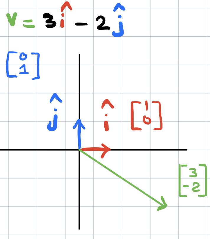
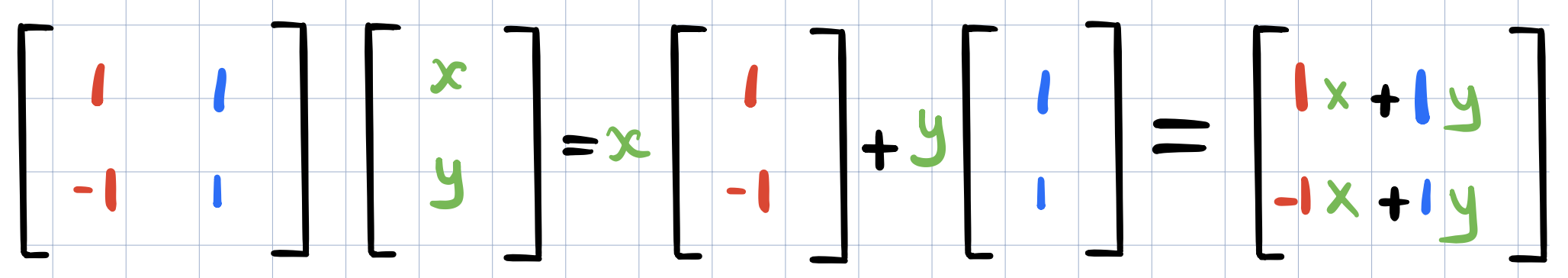
Suppose we want to find out where the vector \(v=(3,2)\) will land after some linear transformation. We can multiply the x-coordinate of \(v\) by the transformed \(\widehat{i}\) coordinates and similarly, multiply the y-coordinate of \(v\) by the coordinates of the transformed \(\widehat{j}\).
To write things numerically, the convection is to arrange the coordinates of these vectors as columns in a 2x2 matrix and then to put the matrix to the left of the vector (just like functions!)
Multiple Linear Transformations
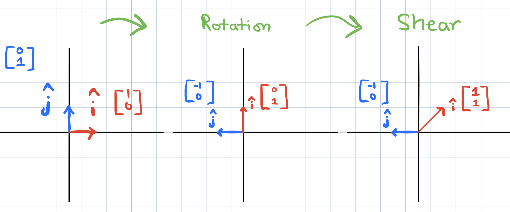
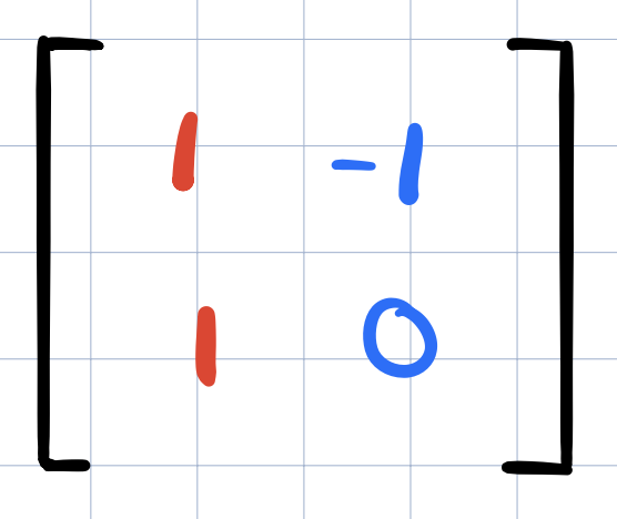
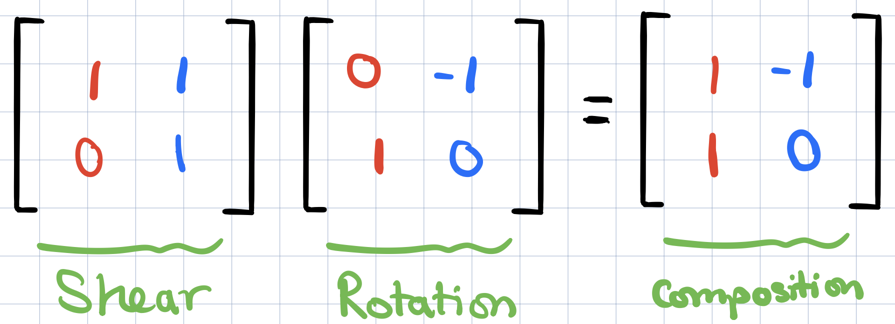
What if we wanted to apply not just one linear transformations but multiple linear transformations? For example, suppose we want to apply a rotation followed by a shear transformation (see above). It turns out that the end result is still another linear transformation recorded in the following matrix,
This new linear transformations is called the composition of the two transformations that we applied (rotation + shear). One way to think about the new matrix is as follows: if we were to take some vector and then pump it through the rotation and then the shear. The long way to compute where it ends up is first to multiply this vector by the rotation matrix on the left and then whatever you get and multiply that on the left by the shear matrix.
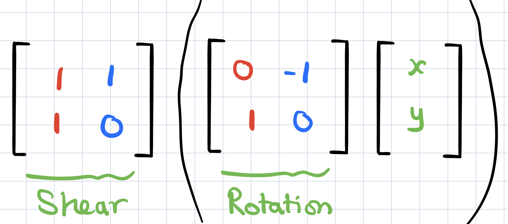
This is what it means to apply a rotation then a shear to a given victor and whatever we get should exactly the same as applying this vector by the new composition matrix.
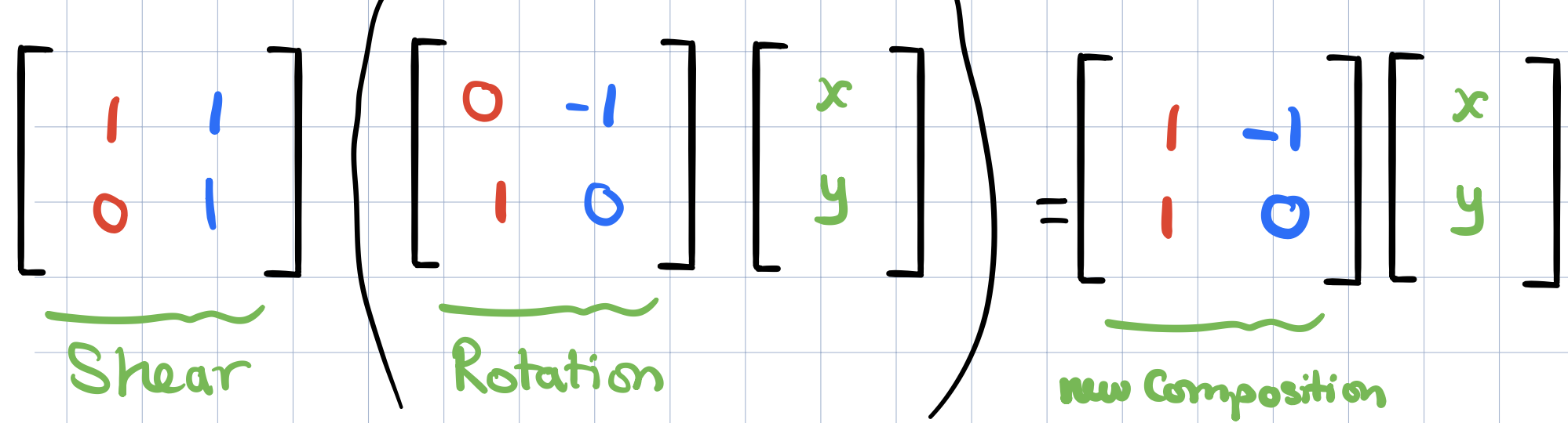
Since this new matrix is supposed to capture this overall effect of applying a rotation and then a shear, it should be reasonable to call this new matrix as the “product” of the original two matrices.
One thing to always remember is that the multiplying two matrices like the above has the geometric meaning of applying one transformation then another. And the reason why we apply the most right matrix first is just following the function notation In \(f(g(x))\), we apply g and then \(f\).
Multiplying Matrices Numerically
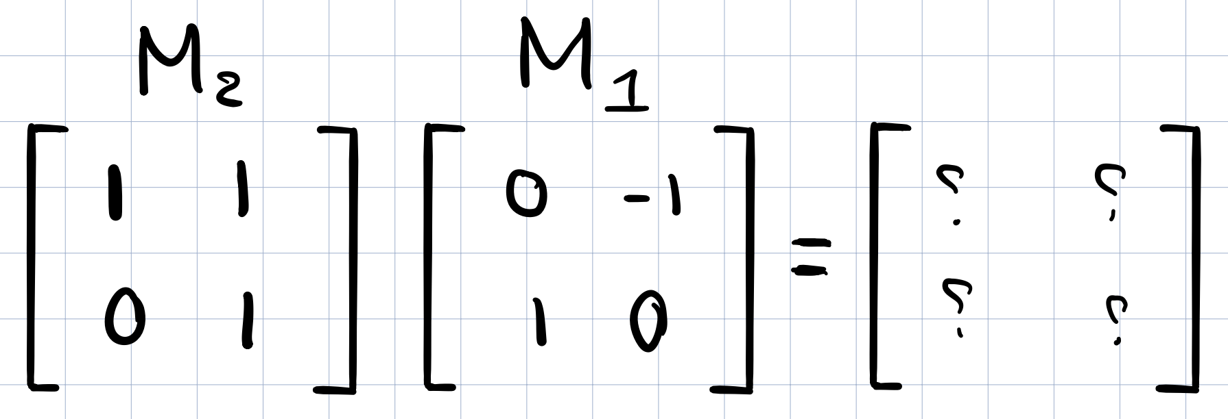
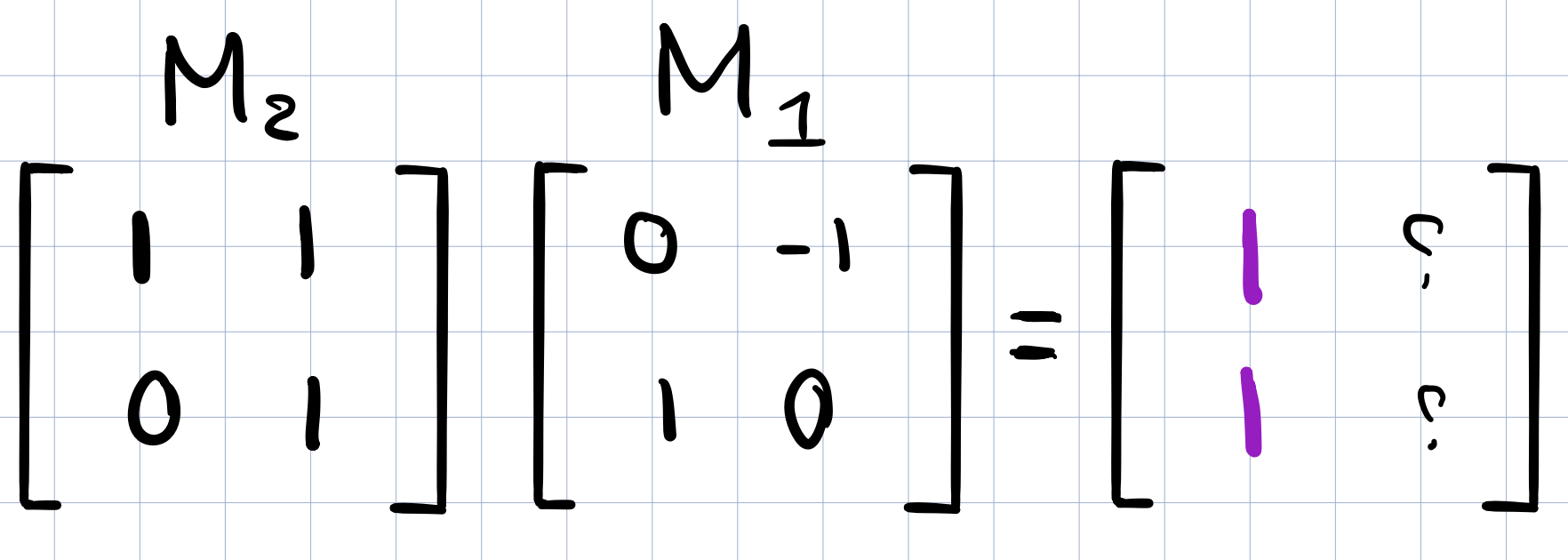
Let’s carry out the multiplication numerically without visualizing it. First we will need to know where \(\widehat{i}\) will land. By definition we know that after applying \(M_1\) above, the new coordinates of \(\widehat{i}\) are captured by the first column of the \(M_1\) matrix and similarly for \(\widehat{j}\). (Recall that the linear transformation matrix records the coordinates of where the two basis vectors have landed).
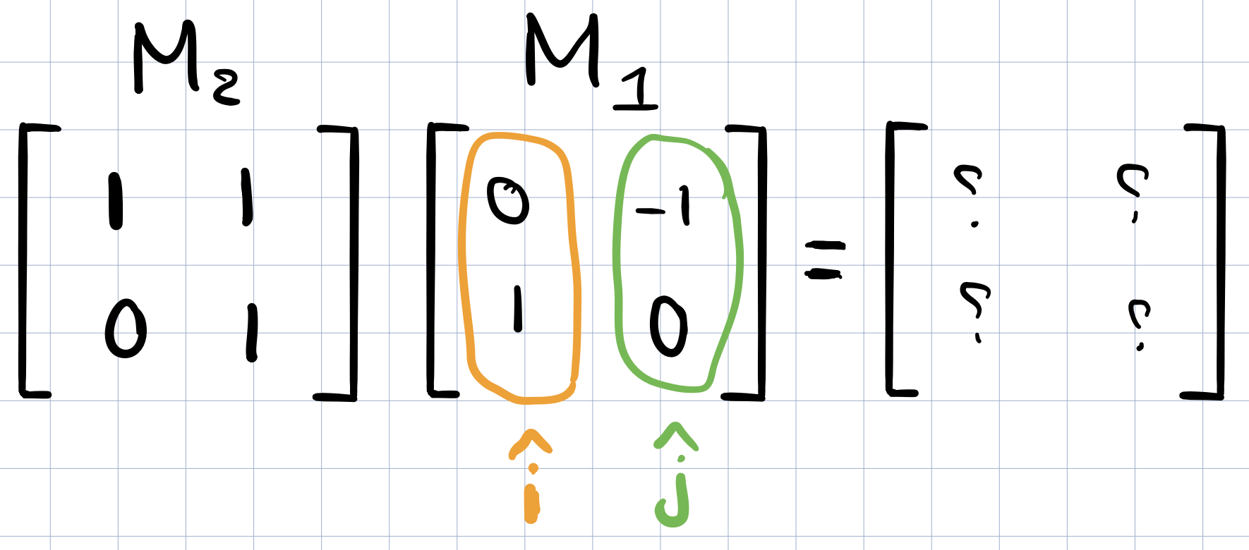
Let’s see what happens after applying the transformation \(M_2\) on the vector (0,1). This can be done by multiplying the x-coordinate of that vector by the first column of \(M_2\) and then similarly multiply the y-coordinate by the second column. (similar to what we learned in the previous video/post)
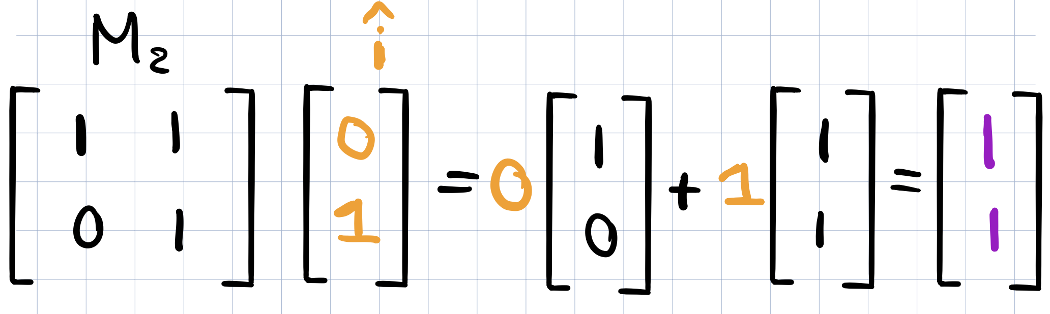
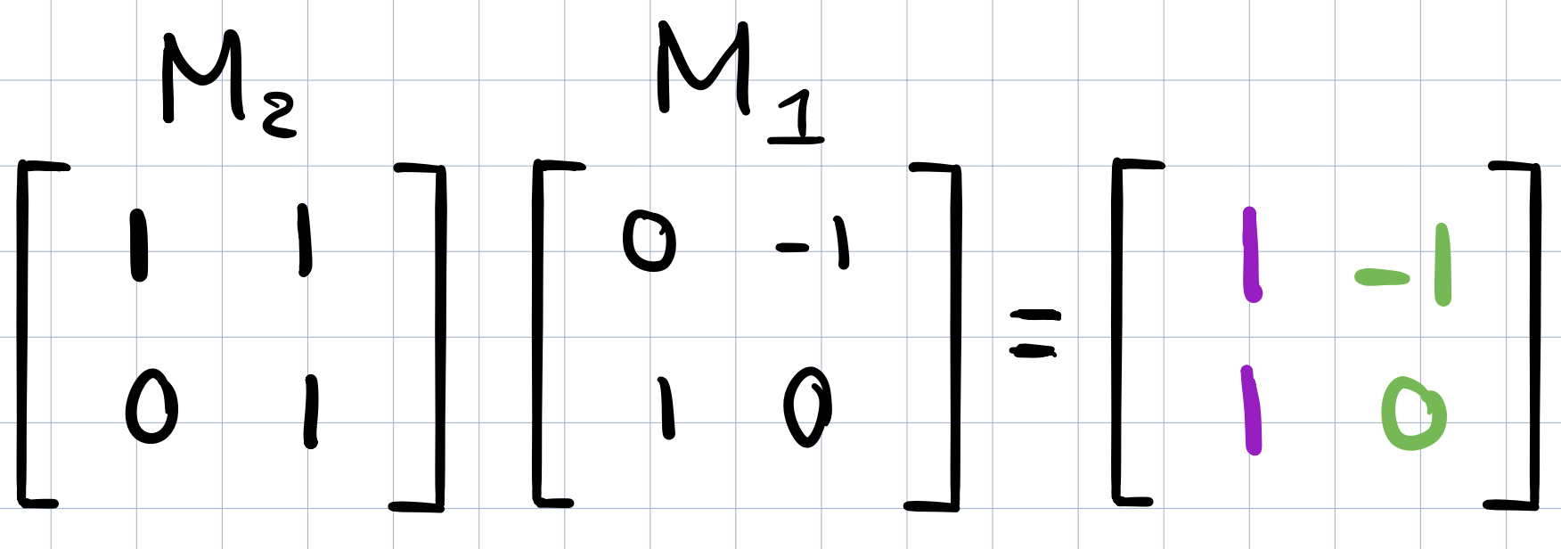
The resulting vector is the first column of the composition matrix below!
Next, we will apply \(M_2\) on the transformed \(\widehat{j}\) vector similar to what we did above for \(\widehat{i}\)
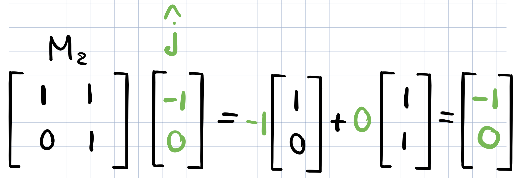
And the resulting vector will be the second column of the new composition matrix!
Properties of Matrix Multiplication
Does the order matter? Does \(M_1M_2 = M_2M_1\)? We can see this by visualizing the transformations. Take a vector and rotate it with the rotation from the above example and then apply the shear from the previous example as well. Take the same vector and apply shear transformation this time before applying the rotation. Do we get the same vector? no. It is so easy to see this with transformations rather than figuring out this numerically!
What about associativity? Does \((AB)C=A(BC)\)? Carrying this out numerically, it is not intuitive and messy! Visualizing this with transformations, it is actually really easy to see that it is true!
3D
The same concept applies to 3 dimensions and the video “chapter 5: Three dimensional linear transformations” has really great animations to show different transformations in 3D.