These are notes I took while watching the series The Essence of Linear Algebra by 3Blue1Brown.

Transformations

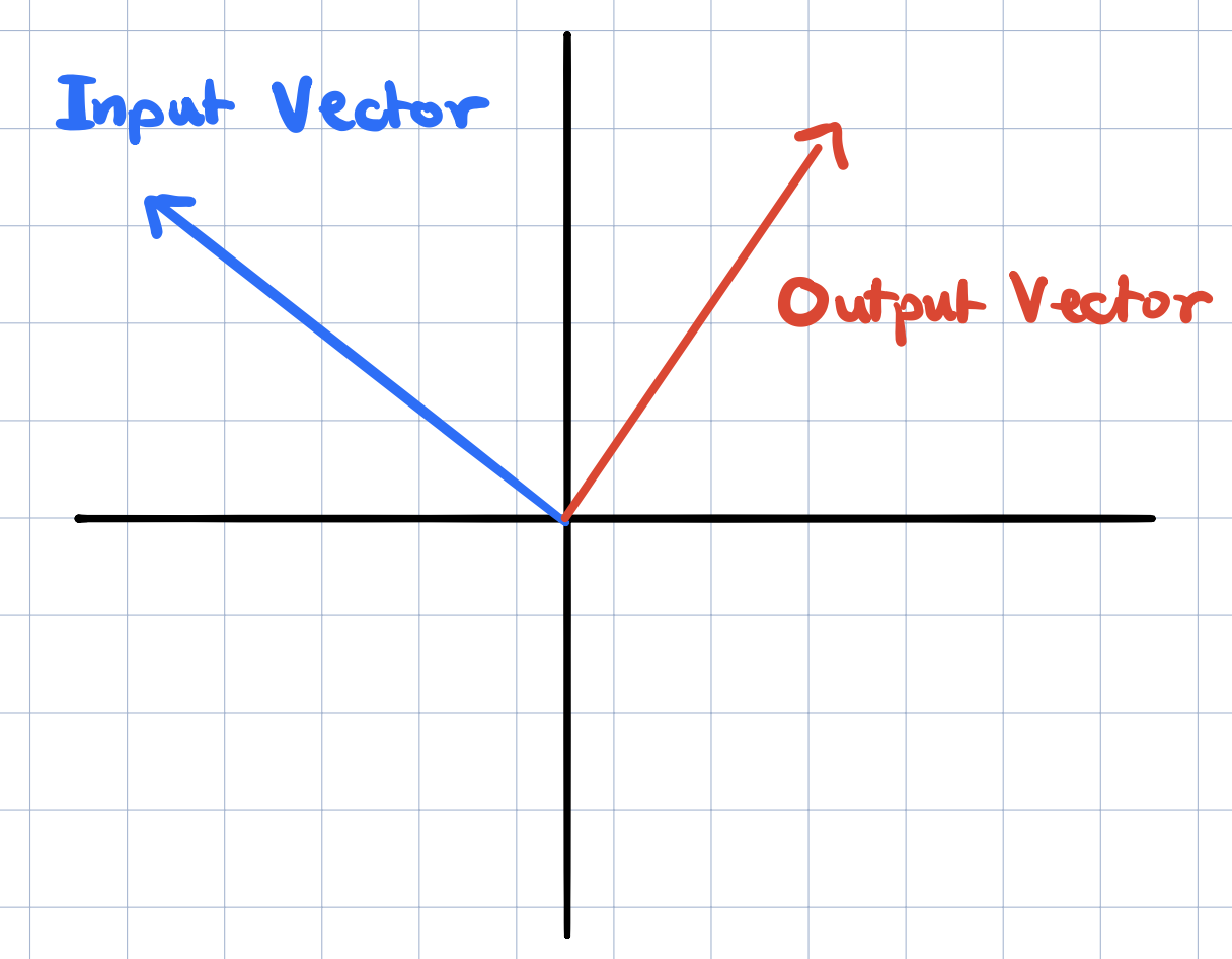
So what does transformation mean? A transformation takes a vector as an input and outputs another vector so it’s just a function. So why didn’t we call it a function? This is because the word transformation suggests movement. We’re imagining that this input vector is moving over to the output vector. Of course, when transforming vectors, it is much nicer to use the trick from last time where we think of the vector as the point where its tip sits on. This way it is easier to visualize transforming many vectors all at once.

Linear Transformations

Transformations can be pretty complex but Linear Algebra is restricted to only linear transformations. Visually speaking a transformation is linear if it has two properties:

All lines must remain lines without getting curved.
The origin is fixed in place.

Describing Linear Transformations Numerically

How do we describe a linear transformation? It turns out that all we need to do is to record where the basis vectors will land and then everything else will just follow. Why is this? From the previous post, we know can write any vector as a linear combination of the basis vector of the vector space. Suppose $v = \begin{bmatrix}3 & -2\end{bmatrix}$, then we know that we can write $v$ in terms of $\widehat{i}$ and $\widehat{j}$ as shown below.

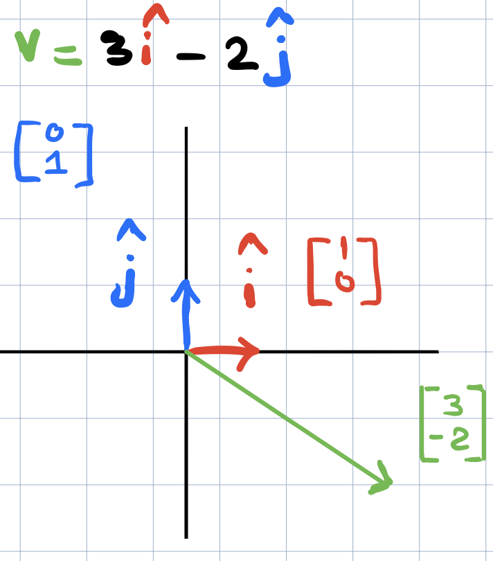
Writing this again, we have

$$$$ \begin{align*} v &= 3\widehat{i} - 2\widehat{j} \\ \begin{bmatrix} 3 \\ -2 \end{bmatrix} &= 3 \begin{bmatrix} 1 \\ 0 \end{bmatrix} - 2 \begin{bmatrix} 0 \\ 1 \end{bmatrix} \end{align*} $$$$

After applying the transformation on $\widehat{i}$ and $\widehat{j}$, we can now find out where $v$ will land by writing $v$ as a linear combination of the transformed vectors $\widehat{i}$ and $\widehat{j}$.

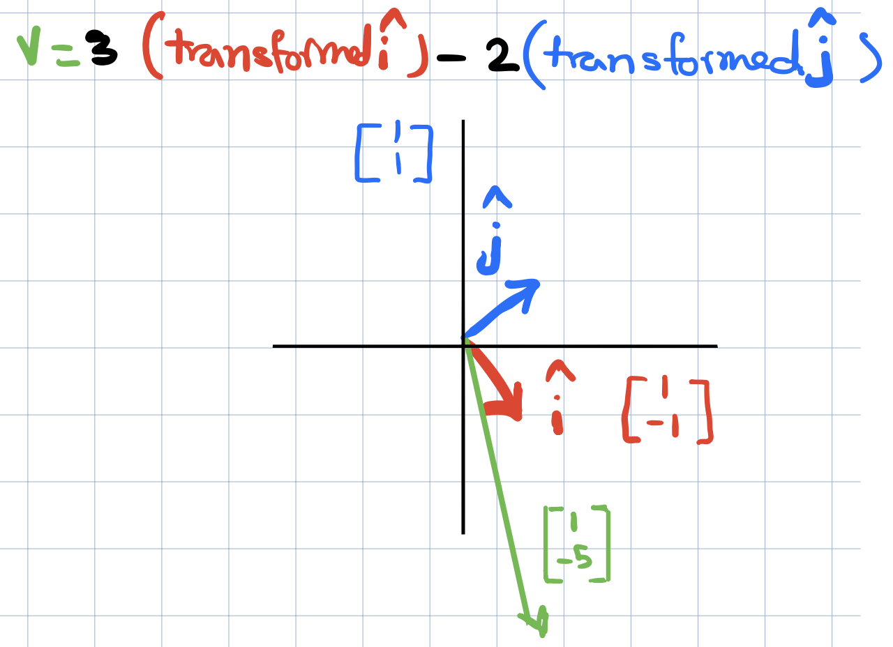
and now we can just know where $v$ will land based on where $\widehat{i}$$and$\widehat{j}$$ landed after the tranformation. We can write,

$$$$ \begin{align*} \text{transformed (} v) &= 3\text{ (transformed }\widehat{i}) - 2 \text{ (transformed }\widehat{j}) \\ &= 3 \begin{bmatrix} 1 \\ -1 \end{bmatrix} - 2 \begin{bmatrix} 1 \\ 1 \end{bmatrix} \\ &= \begin{bmatrix} 1 \\ -5 \end{bmatrix} \end{align*} $$$$

Representing the transformation with a Matrix

So from the above we saw how a two dimensional linear transformation is completely described by four numbers. The two coordinates for where $\widehat{i}$ lands and the two coordinates for where $\widehat{j}$ lands and this is pretty cool! Here is a cooler thing. We can package these coordinates into a two-by-two grid of numbers (a Matrix!)

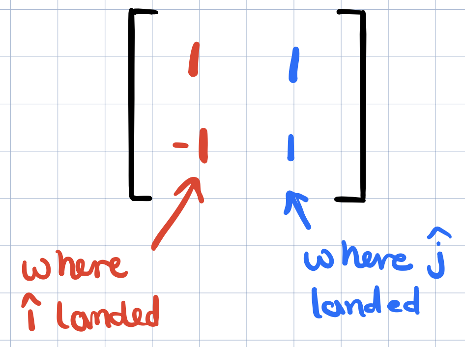
The first column will be where $\widehat{i}$ landed and the second column will be where $\widehat{j}$ landed. So now when we apply the transformation to some vector $v=(x,y)$, what do we get?

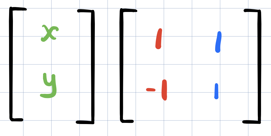
We’ll multiply the $x$ coordinate with the transformed $\widehat{i}$ vector and similarly multiply the $y$ coordinate with the transformed $\widehat{j}$ coordinate.

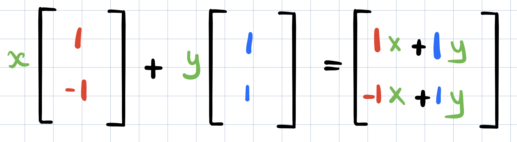
and now we can re-arrange the matrix position to put it on the left of the vector below,

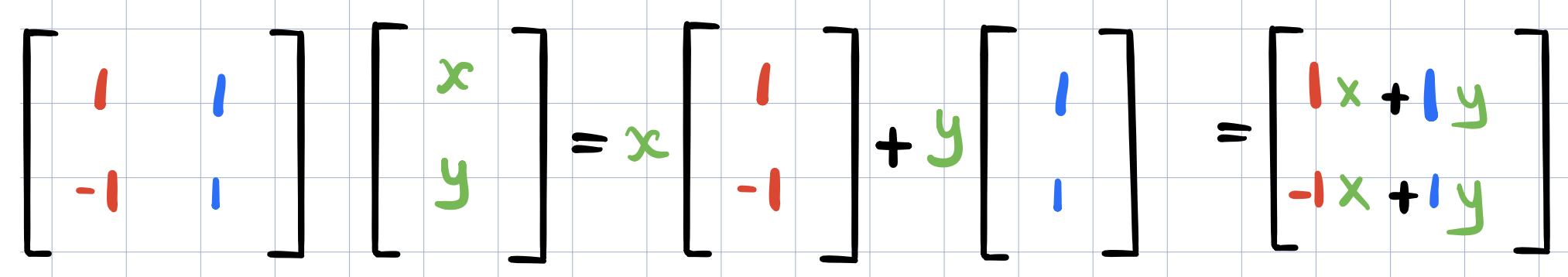
And this is way more fun than just memorizing how matrix multiplication works. These matrix columns are just the transformed versions of your basis vectors and the resulting vector is just a linear combinations of these two vectors.

More Example Transformations

TODO: Rotations and Shear. (the video shows really beautiful animation for the examples)

References

Essence of Linear Algebra by 3Blue1Brown