 Given an array with \(n\) elements. Quicksort is a fabulous divide-and-conquer sorting algorithm with a worst-case running time of \(O(n^2)\) and an expected running time of \(O(n\log(n))\). The main technique or idea used in quicksort is choosing a pivot, and then partitioning the elements around this pivot.
void quicksort(int *a, int first, int last, int n) {
    if (first < last) {
        int p = partition(a, first, last, n); /* partition index */
        quicksort(a, first, p - 1, n);
        quicksort(a, p + 1, last, n);
    }
}
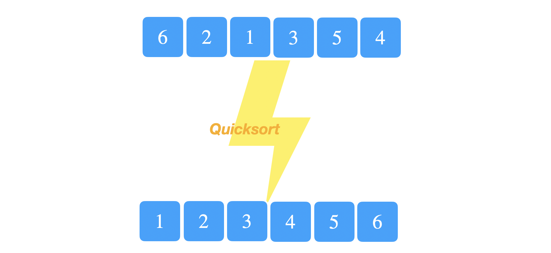
Example
Here, we have an unsorted array of 6 elements.

Suppose the first random pivot was 3.

We will partition the array such that all the elements less than or equal to 3 will be on the left and all the elements larger than 3 will be on the right. At this point, we have two new subproblems, the left and right subarrays. We recursively call quicksort on each half.

Next, suppose the next random pivot was 2 for the left subarray and 5 for the right subarray.

We repeat the same process of partitioning around each pivot.
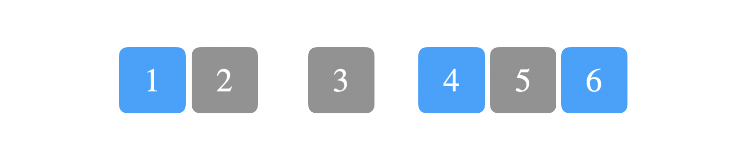
We now call quicksort again on each new subarray, highlighted in blue.

The base case of the recursion is reaching an array of size 1 (\(first < last\) is not true). In this case, we do nothing since an array of size 1 is already sorted. So, it’s time to combine all these smaller solutions in one array. However, unlike Mergesort, we’re doing all the partitioning work in place and so naturally we’re done.

Partition
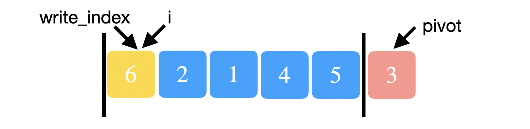
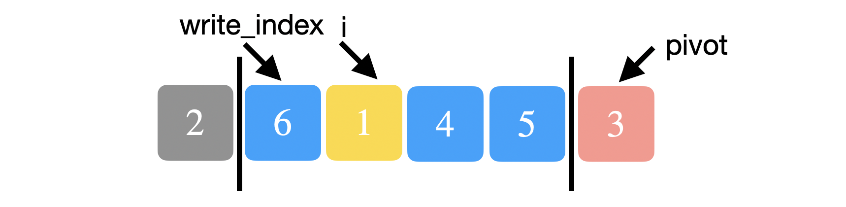
The most critical or the only thing we really do in Quicksort is partitioning the array around a chosen pivot. There isn’t anything cuter than partition. The implementation trick to partition is to move the pivot to the end of the array. So, for the above example, we will swap 3 and 4 and set the pivot to be the last index of the array.

We will also keep track of an index, \(i\), to iterate through the array. At each iteration, we will compare the element at index \(i\) with the the pivot. The trick to partition is keeping track of another index, \(write{\_}index\). Whenever we see an element that is less than the pivot, we swap it with the element at \(write{\_}index\) and increment \(write{\_}index\). The intuition here is that we want all the elements less than the pivot to be stored below \(write{\_}index\).
Initially, \(i=0\) and \(write {\_} index =0\). We compare \(array[i=0]=6\) to the pivot, 3. Since 6 is not smaller, we just increment \(i\).
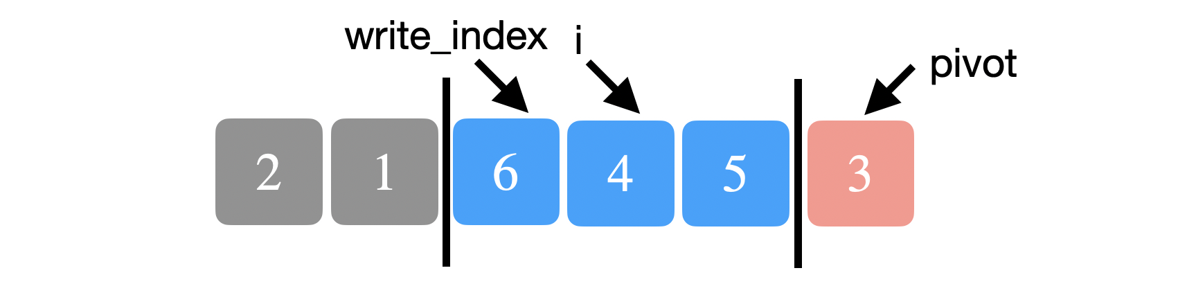
Next, we have \(i=1\) and \(write{\_}index =0\). We compare \(array[i=1]=2\) to the pivot, 3. 2 is smaller so we swap 2 and 6 and then increment both \(write{\_}index\) to 1 and \(i\) to 2.
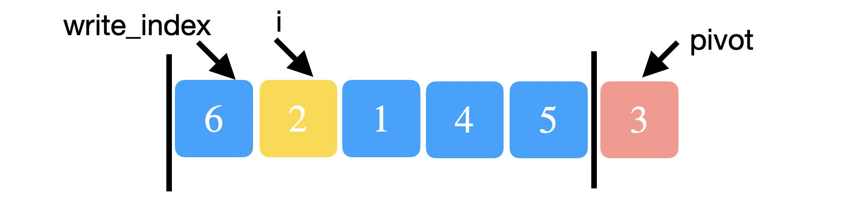
Notice below that 2 and 6 are now swapped. \(array[write{\_}index = 1] = 6\) and \(array[i = 1] = 1\). 1 is also smaller than 3 so we swap 6 and 1 and increment both \(i\) and \(write{\_}index\).
You can see below that the elements before \(write{\_}index\) are indeed smaller than the pivot. We repeat the same process of comparing the current element at \(i\) to the pivot. 4 is not smaller than 3 so we just increment \(i\).
We repeat the above process until we reach the pivot and we stop. The very last thing we want to do is to place the pivot back in its correct place. We swap the pivot with the element at \(write{\_}index\).
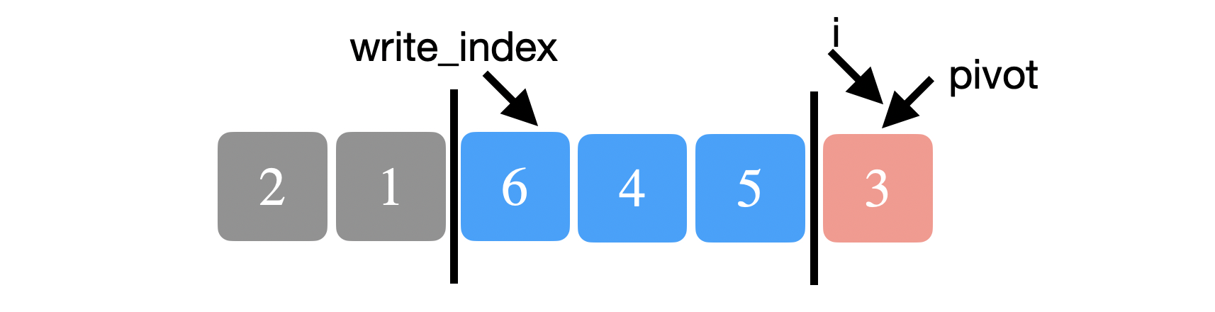
The write_index is now our real pivot that we want to return to quicksort.

Implementation
int partition(int *a, int first, int last, int n) {
    srand(time(NULL));
    int random_pivot = rand() % (last+1-first) + first;

    // move the pivot to the end of the array
    swap(&a[random_pivot], &a[last]);
    int pivot = last;

    int write_index = first;
    for (int i = first; i < last; i++) {
        if (a[i] < a[pivot]) {
            swap(&a[i], &a[index]);
            write_index++;
        }
    }
    swap(&a[pivot], &a[write_index]);
    return write_index;
}Correctness of partition
The proof is done with a standard loop invariant. For partition above, we want to establish the following invariant:
For any index \(k\) in the array:
- If \(write{\_}index \leq k \leq i\), then \(array[k] \leq array[pivot]\). (Remember we’ve already said any element below \(write{\_}index\) is less than the pivot).
- If \(i < k \leq pivot - 1\), then \(array[k] \leq array[pivot]\).
- If \(i == pivot\), then \(array[k] = array[pivot]\).
Proof is in CLRS ;)
Worst-case running time analysis
What’s the worst possible input to quicksort? Suppose we always pick the pivot to be the largest or the smallest element in the array. Then, we will have two subproblems, one of size \(n-1\) elements and the other of size \(0\). We know partition runs in linear time. If \(T(n)\) was the total time it takes to run quicksort then,
This recurrence has the solution \(T(n)=O(n^2)\) which is the worst-case running time of quicksort. Intuitively, if we always choose either the smallest or the largest index as a pivot, then we will be making \(O(n)\) calls to partition. Partition takes linear time and so the total running time will be \(O(n^2)\).
Best running time analysis
How good can quicksort be? Suppose that the pivot is always chosen to be the middle element in the array. Then our recurrence would look like the following,
By the master theorem, the solution is \(T(n) = O(n\log(n))\). Intuitively, if we always partition the array around the middle element, we will need to make \(O(\log(n))\) calls to partition and therefore, we get \(O(n\log(n))\) as the overall runtime.
Expected running time analysis
This analysis depends on the important idea that quicksort is dominated by the number of comparisons it makes while partitioning the array (proof in CLRS). Moreover,
| for any given pair of elements, \(x\) and \(y\). We know that \(x\) and \(y\) are compared at most once during quicksort. |
Proof: \(x\) and \(y\) are only ever compared if one of them is chosen as a pivot. Moreover, once we do the comparison, the pivot will be excluded from all future calls to partition and so \(x\) and \(y\) will not be compared to each other again.

So, how do we count the number of comparisons quicksort makes? Let \(A = \\{z_1, z_2, ..., z_n\\}\) be an array of distinct elements, such that \(z_i\) is the \(i\)th smallest element. Let \(X\) be the total number of comparisons quicksort makes and let \(X_{ij}\) be an indicator random variable such that,
Since we make at most one comparison between each pair, we can write \(X\) as follows
We are interested however in the expected number of comparisons. Therefore, we take the expectation of both sides to see that,
How to compute \(P(X_{ij}=1)\)?
Let \(Z_{ij} = \\{z_i,...,z_j\\}\) be the set of elements between \(z_i\) and \(z_j\) inclusive.

What is the significance of \(Z_{ij}\) to the probability of \(x_i\) and \(x_j\) being compared?
Suppose we pick a pivot that’s not in \(Z_{ij}\), then this event doesn’t affect the chance of \(z_i\) and \(z_j\) being compared. However, if the choice of pivot was from the set \(Z_{ij}\) then we have two cases:
- If the pivot was \(z_i\) or \(z_j\) then the \(z_i\) and \(z_j\) will be compared.
- If the pivot was any other element in \(Z_{ij}\), then \(z_i\) and \(z_j\) will be partitioned in separate halfs and will never be compared. Based on the above, only two choices out of \(j-i+1\) choices will lead to having \(z_i\) and \(z_j\) be compared. Therefore,
Apply this back in the previous expectation,
Using the harmonic series,
We can further simplify the expectation to be
Thus, the expected running time of quick sort is \(O(n\log(n))\) when the elements are distinct.
References
- CLRS Chapter 7
- CS161 Stanford