What is a Random Variable?
A random variable is a real-valued function defined on a sample space. Why define a random variable? sometimes instead of being interested in the individual outcomes of an experiment, we are interested in some groups of the outcomes or more formally some function of the outcome.
Example 1:
Suppose we’re interested in counting the number of heads in \(5\) trials of flipping a coin. We can define a random variable \(Y\) to represent the number of heads in 5 trials. Using \(Y\), we can now refer to the probability of seeing two heads in 5 trials as \(P(Y=2)\). This is much simpler that listing the exact outcomes that we’re interested in. (\(\{H,H,T,T,T\},\{H,T,H,T,T\},...\}\)).
Example 2:
Suppose we roll two dice and we’re interested in the sum of the two dice. We define a random variable \(X\) to be the sum of two dice (function of outcomes). We can now refer to the probability that the sum of the dice is 7 as \(P(X=7)\). This is much simpler that saying that we want the probability of seeing any of these outcomes: \((3,4),(4,3),(2,5),(5,2),(1,6),(6,1)\).
Discrete Random Variables
If our random variable takes on countable values \(x_1, x_2, x_3,...,x_n\), we call it a discrete random variable.
Probability Mass Function
Suppose we have a random variable \(X\) that takes on a discrete values in \(R_X = \{k_1, k_2,...,k_n\}\). Define the probability mass function \(p_X(k)\) to be the probability that \(X\) takes on a particular value \(k\). In other words, the PMF is defined as
Furthermore, the PMF of \(X\) satisfies
This also means that for any value \(k\) that is not in \(R_X\), we have \(p_X(k) = 0\),
We can also refer to \(p_X(k)\) as just \(p(k)\) if the random variable is clear from the context.
Example 2:
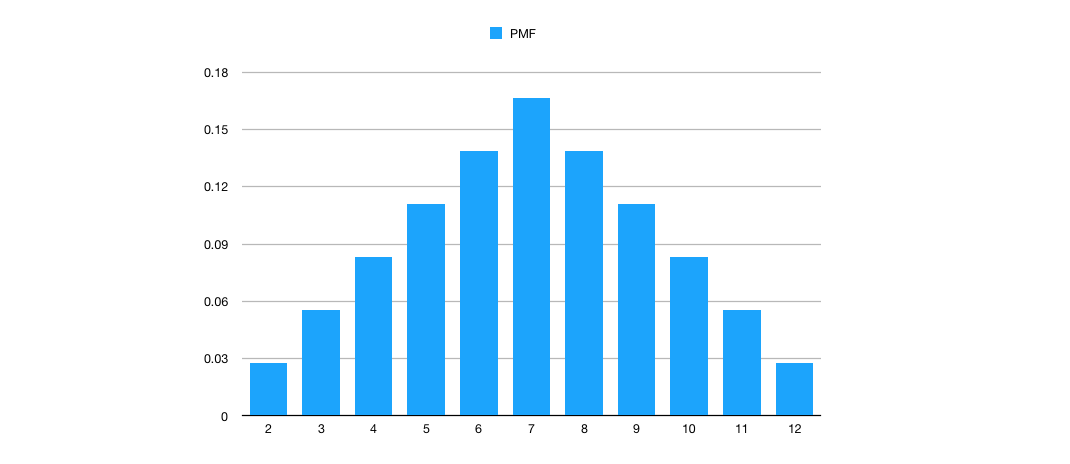
Suppose we roll the two dice again from example 2. Define a random variable \(X\) to be to the sum of the two dice. We know \(R_X = \{2,3,4,5,6,7,8,9,10,11,12\}\). Below is a graph of the \(PMF\) of \(X\), \(p_X(k)\) for all values in \(R_X\).
Cumulative Distribution Function
Suppose we’re interested in the probability that a random variables, \(X\), is less than or equal to a particular value, \(C\). One way to do this is to sum all the probabilities for all the values that \(X\) can take up to \(C\). An easier way to do this is to use the cumulative distribution function (CDF) that gives the probability that \(X\) is less than or equal to a particular value, specifically
For a discrete random variable, this will be just the sum of all variables
Expectation
The expectation or expected value of a random variable \(X\) is defined as:
In other words, the expected value is a weighted average of the value of the random variable (values weighted by their probabilities).
Example 4:
Suppose we roll two dice again from example 2 and 3. Define a random variable \(X\) to be to the sum of the two dice. We can use our PMF from the previous section to compute the expected value as
Expectation of a function of a random variable
Suppose we have a random variable \(X\) and we have a function \(g\) where \(g\) is real-valued function. Suppose we want to calculate the expected value of \(g(X)\). Define
PROOF?
Example 5:
Suppose we roll a die and define \(X\) to be the value on the die. Define a new random variable \(Y\) to be \(X^2\). What is \(E[Y]\)?
Using the above, \(E[Y] = E[X^2] = \sum_i (k_i^2)p(k_i) = 1/6*(1+4+9+16+25+36) \approx 15.167\)
Linearity of Expectation
Expectation of the sum of two random variables is the sum of expectation of the two random variables.
Example 6:
Suppose we roll a die and let \(X\) be a random variable representing the outcome of the roll. Suppose also that you will win a number of dollars equals to \(3X+5\). What is the expected value of your winnings? We can let \(Y\) be a random variable representing our winnings. Now we have
However using the linearity of expectation, we know that \(E[X]=3.5\). Therefore we could do the following:
Example 7:
Suppose we roll two dice again and we’re interested in the expectation of the sum of two dice. We calculated this value previously in example 4 using the PMF. Let’s use the second property of expectation. Let \(X_1\) be a random variable representing the value of the first die and \(X_2\) be a random variable representing the sum value of the second die. Let the sum of the two dice be \(X_1 + X_2\).
Example 8: St. Petersburg Paradox
A fair coin comes up heads with \(p = 0.5\). We flip the coin until we see the first tails. We will then win \(2^n\) dollars where \(n\) is the number of heads seen before the first tail. How much would you pay to play?
Let’s define the following random variables:
Let \(Y\) be the number of “heads” before the the first “tails”.
Let \(W\) be a random variable representing our winnings. \(W = 2^Y\).
What is the probability of seeing \(i\) heads before seeing the first tail on the \(i+1\)th trial? \(P(Y = i) = (1/2) * (1/2) * ... = (1/2)^{i+1}\). This is because we stop at the \(i+1\) flip which is a tail. Each outcome has a probability equals to \(1/2\).
What is the expected value of our winnings?
Example 9: Roulette
Consider an even money bet (betting “Red” in Roulette). \(p=18/38\) you win \(Y\) dollars, otherwise \(1-p\) you lose \(Y\) dollars. Consider the following strategy:
- Let \(Y=1\).
- Bet \(Y\).
- If win then stop.
- Else let \(Y=2Y\) go to step 2.
What is the expected value of our winning?
Define \(Z\) to be our winnings until we stop.
References
My study notes from CS109 http://web.stanford.edu/class/archive/cs/cs109/cs109.1188//
Specifically: http://web.stanford.edu/class/archive/cs/cs109/cs109.1188/lectures/06_random_variables.pdf