Problems with greedy solutions might have really simple and straight forward solutions however, they are really hard to reason about. This is why greedy algorithms are generally taught toward the end of an algorithms class. One classic problem with a greedy solution is the activity selection problem. In this problem, we are given a list of activities, each with a start time, \(t_i\), and a finish time, \(f_i\), and we would like to pick a set of activities such that the total number of activities is maximized with the constraint that no two activities can overlap.
Greedy Solution
As we said earlier, typically greedy solutions are super straight forward and easy. For the activity selection problem, one approach that works is to simply select the activity with the earliest finish time at each step until we run out of activities.
Example
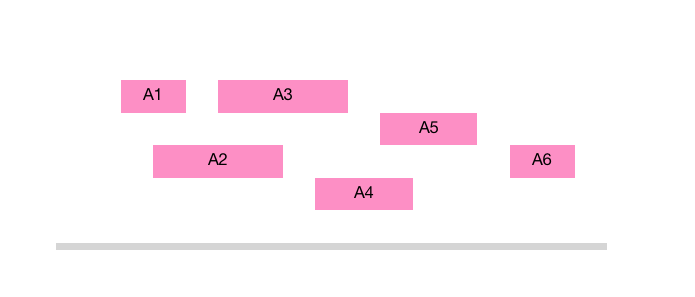
Suppose we have the following activities:
 Based on our strategy, we will pick \(A1\) first. We will skip \(A2\) since it violates the condition of not having overlapped activities. We will then go on to pick \(A3\), \(A5\) and \(A6\).
Implementation
typedef struct activity {
    int start_time;
    int finish_time;
} activity;
bool custom_sort_by_finish_time(const activity &a, const activity &b) {
    return a.finish_time < b.finish_time;
}
std::vector<activity> select_maximum_activities(std::vector<activity> activities) {
    std::sort(activities.begin(), activities.end(), custom_sort_by_finish_time);
    std::vector<activity> picked;
    for (int i = 0; i < activities.size(); i++) {
        if (activities[i].start_time >= picked[picked.size()-1].finish_time) {
            picked.push_back(activities[i]);
        }
    }
    return picked;
}
Correctness Proof
This is the most interesting part of any greedy algorithm! why does it work? To prove the correctness of greedy algorithms, we want to prove that as we select activities, we are not ruling out the optimal solution. So, each decision we make doesn’t affect our ability of reaching out an optimal solution.
This should sound very familiar. We have a base case where we start with an empty set of activities and then we want to prove that each selection we make doesn’t rule out an optimal solution. What proof method should we use? of course, Induction.
Proof By Induction:
Inductive Hypothesis: After adding the \(t\)‘th activity, there is an optimal solution that extends our current solution.
Base Case: When we add the zero’th activity, there exists an optimal solution that extends the current solution which contains no activities yet.
Inductive Step:
Let \(k\) be a natural number and suppose we’re about to add the \(k\)‘th activity and that our inductive hypothesis holds for \(k-1\), meaning that we didn’t rule out an optimal solution yet and that there is some optimal solution \(T^*\) that extends the \(k-1\) choices we’ve made so far. We’re about to select our \(k\)‘th activity.
Our greedy algorithm picks the next activity with the earliest finish time such that it doesn’t overlap with any of the \(k-1\) activities we’ve selected so far. Let our selection be \(a_j\) for some natural number \(j\). There are two cases
Case 1: \(a_j\) is in the optimal solution so \(a_j \in T^*\). yay, we didn’t rule out the optimal solution and we’re done!
Case 2: \(a_j\) is not in the optimal solution so \(a_j \not\in T^*\). In this case, some other activity was selected instead of \(a_j\). Let that activity be \(a_k\). Let’s consider swapping \(a_j\) and \(a_k\) to create a new set of activities, \(T\).
We claim that \(T\) is allowed and optimal. First, we know that \(a_j\) has a smaller finish than \(a_k\) because our greedy algorithm selects the activity with the earliest finish time. Therefore, \(a_j\) doesn’t conflict with anything chosen after \(a_k\). From this we see that \(T\) also has the same number of activities as \(T^*\) and therefore, we can conclude that \(T^*\) is optimal.
Conclusion:
After adding the last activity, we will have an optimal solution that extends our current choices. Our current choices or solution is the only solution that extends the current solution and therefore, our current solution is optimal. \(\blacksquare\)
Running Time
If we need to sort the activities, then it will be \(O(n\log(n))\). If it’s sorted, then we’re only doing a linear scan of activities and therefore, the running time is \(O(n)\).