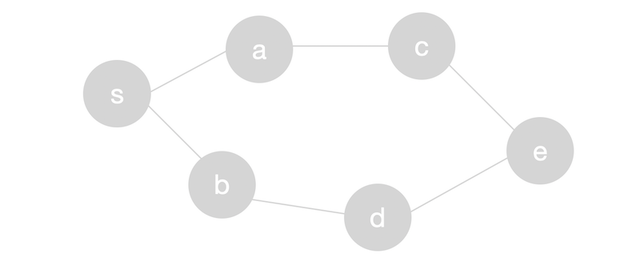
Breadth first search is a useful and widely used algorithm in graph traversal problems. Let \(G = (V, E)\) be a graph consisting of \(V\) vertices and \(E\) edges and let \(s\) be the source vertex where we will start the traversal from. The key thing about breadth first search is that it explores the vertices closest (in terms of the number of edges) to the source vertex first. We start by looking at \(s\)’s neighbors. These vertices are the closest vertices to \(s\) and have distance 1 from \(s\). We then explore each adjacent vertex to all the neighbors of \(s\). These vertices will have distance 2 from \(s\).
In other words, breadth first search explores the graph in layers. The immediate neighbors are in layer 1 and have distance 1 to the source vertex. The vertices in layer 2 have distance 2 to the source vertex and so on. Given a layer, all the vertices in that layer have the same distance to the source vertex. It turns out that breadth first search also finds the the shortest paths from the \(s\) to every other vertex in the graph in terms of the number of edges between \(s\) and each vertex. We’ll prove this later!
Implementation Details
How could we implement a breadth first search on \(G\)? We want to explore the vertices closest to \(s\) first. To do so, we will maintain the following data structures:
-
A queue. We want to explore the nodes closest to \(s\) first. We know that a queue maintains the property that a node inserted first will be popped/explored first. We will also use the queue to keep track of the distance of each vertex to \(s\). Initially we will enqueue \(s\) with distance 0. When we enqueue new nodes, we will also enqueue their distance to \(s\) which is just their parent’s distance plus 1.
-
A set or an array that keeps track of the visited nodes. Remember that \(G\) might contain cycles and so we want to make sure that we explore each node once only.
-
A set or an array that keeps track of the parent nodes. This is optional and only needed if we want to recover the path from \(s\) to every other node in \(G\).
Example
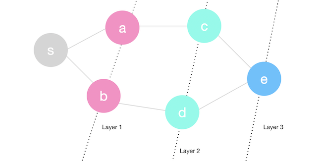
Let’s explore the graph above. We will start by popping \(s\) from the queue with its distance 0. We will then enqueue the neighbors of \(s\) along with distance 1 and also mark them visited. We could also use the parent array to indicate that \(s\) is the parent of \(a\) and \(b\). At this point, we have \(a\) and \(b\) in layer 1 with distance 1. This information will not change in any future iteration.
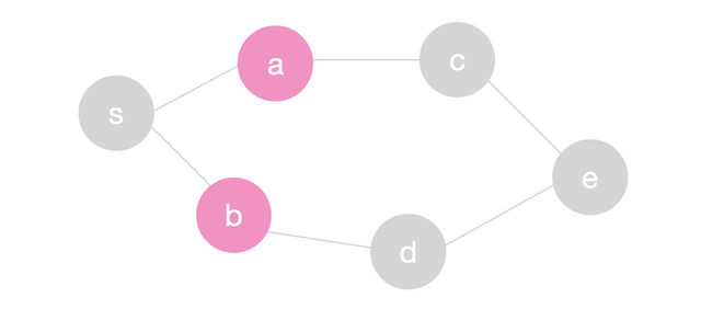
Next we will we will pop \(a\) from the queue. We will traverse \(a\)’s neighbors \(s\) and \(c\) but \(s\) will be ignored since it was visited before. When we add \(c\) to the queue, we will also push distance 2 which indicates that \(c\) is in layer 2 or is two steps away from \(s\). We also mark \(c\)’s parent as \(a\). Next we will we will pop \(b\) from the queue and and push \(d\) on the queue with distance 2. \(c\) and \(d\) are colored in green below to indicate that they are in a new layer (distance = 2).
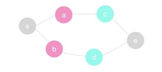
We will repeat the same process until the queue is empty and we have reached every node reachable from \(s\).
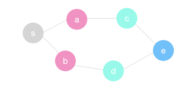
Notice now how the nodes are organized in layers in terms of the distance from \(s\) (number of edges).
Implementation
int bfs(int start, int end, std::vector<std::vector<int>>& graph) {
    std::queue<int> q;
    q.push(start);
    // another queue to push the distances down (bfs works in layers)
    std::queue<int> qd;
    qd.push(0);
    // visited array so we don't revisit nodes
    std::vector<int> visited(graph.size(), false);
    visited[start] = true;
    // parent array to print the path
    std::vector<int> parent(graph.size(), -1);
    int d = 0;
    while (!q.empty()) {
        int v = q.front();
        d = qd.front();
        qd.pop();
        q.pop();
        if (v == end) {
            break;
        }
        for (int i = 0; i < graph[v].size(); i++) {
            int u = graph[v][i];
            if (visited[u] == false) {
                q.push(u);
                parent[u] = v;
                visited[u] = true;
                qd.push(d+1);
            }
        }
    }
    // print path (reversed)
    while (end != -1) {
        printf("%d ", end);
        end = parent[end];
    }
    printf("\n");
    return d;
}Why does breadth first search find the shortest distances?
Intuitively, we know that we explore the vertices in layers starting at \(s\). So if we have a vertex \(x\) in layer \(j\) then we know the distance from \(s\) to \(x\) is \(j\) and that \(x\) can’t have a shorter path to \(s\) because we would have found \(x\) in an earlier layer, right? Below is a proof by induction.
Claim
Let \(G = (V,E)\) be a graph, \(s\) be the source vertex and \(L_i\) to be the \(i\)th layer where \(i\) is a natural number. For all \(i\), \(L_i=\{x \ | \ distance(s,x) = i\}\). In other words, the vertices in layer \(L_i\) have distance \(i\) from \(s\).
Proof:
The proof is done by strong induction.
Base Case:
For \(i=0\), we know that \(L_0=\{s\}\) and we know that \(s\) has distance 0 from \(s\) so we’re done.
Inductive Step:
Let \(j\) be a natural number. In our inductive hypothesis, we will assume that the claim is true for all \(j \leq i\) (strong induction). That is, the vertices in layer \(L_j\) have distance \(j\) from \(s\). We want to prove that our claim is true for \(i+1\). So, for any give vertex \(w\), \(w\) is in \(L_{i+1}\) if and only if \(distance(s,w) = i+1\).
\(\rightarrow\) Suppose that \(w\) is in \(L_{i+1}\), then it must have been added by traversing some edge \((x,w)\) where \(x \in L_i\). We know that the distance from \(s\) to \(w\) is of length \(i\) by the inductive hypothesis. Therefore, we must have \(distance(s,w) \leq distance(s,x)+1\). In other words, the distance from \(s\) to \(w\) can’t be shorter than \(distance(s,x) + 1\) by the definition of shortest paths. Also by the Inductive hypothesis, we know that \(w\) is not in \(L_j\) for any \(j \leq i\) and so we must have \(distance(s,w) > i\). We therefore conclude that \(distance(s,w) = i+1\).
\(\leftarrow\) Next suppose that \(distance(s,w)=i+1\). By the inductive hypothesis, we know that \(w\) must not be in \(L_j\) for any \(j \leq i\). On the shortest path from \(s\) to \(w\), suppose the node preceding \(w\) is \(x\). We must have \(distance(s,x)+1=distance(s,w)\) by the definition of shortest paths. Therefore, \(distance(s,x)=i+1-1=i\). By the inductive hypothesis, \(x\) must be in \(L_i\). By breadth first search, when we scanned \(x\), we looked at each neighbor of \(x\) and \(w\) is a neighbor of \(x\) by the edge \((x,w)\). If \(w\) was not seen before then \(w\) will have distance \(i+1\) and so \(w\) is in \(L_{i+1}\). If \(w\) was already visited, then \(w\) must have been seen in an earlier layer than the current layer \(i\). But that’s impossible since by the inductive hypothesis, \(w \in L_j\) where \(j \leq i\). Therefore, we must have added \(y\) to \(L_{i+1}\).
Conclusion:
For all vertices \(w \in V\), if \(w \in L_j\), then \(distance(s,w) = j\).
Running Time
We visit each vertex at most once only because of the visited array we’re maintaining. That’s \(O(V)\) time. As a result, we also visit the adjacency list of each vertex at most once and that’s \(O(E)\). Therefore, the total time is \(O(V+E)\).