 Let \(G=(V,E)\) be a weighted graph with \(V\) vertices and \(E\) edges. Bellman-Ford is a dynamic programming algorithm that for a given a vertex ,\(v\), finds all the shortest paths from \(v\) to all the other vertices in \(G\).
Motivation
But why another shortest paths algorithms. W’ve already discussed Dijkstra’s algorithm to find the shortest paths which is extremely fast and runs in just \(O(V\log(V)+E)\) time. Unfortunately, Dijkstra doesn’t handle negative edge weights and bellman-ford could! so it’s important to learn what bellman-ford is about!
Optimal Substructure
Since it’s a dynamic programming algorithm, then this means that we must have some optimal recursive substructure where a solution to the problem includes solutions within it to smaller subproblems.
Let \(D[v,i]\) be the length of the shortest path from \(s\) to some vertex \(v\) whose number of edges is at most \(i\). Given that we know \(D[v,i]\) for all \(v \in V\), what can we say about \(D[v,i+1]\)? In other words, given that we know the shortest path using at most \(i\) edges from \(s\) to any vertex in \(G\), what can we say about the length of the shortest path from \(s\) to some vertex \(v\) with at most \(i+1\) edges? Let’s think about this before looking at the answer. Bellman-Ford definitely wasn’t easy for me to think about.
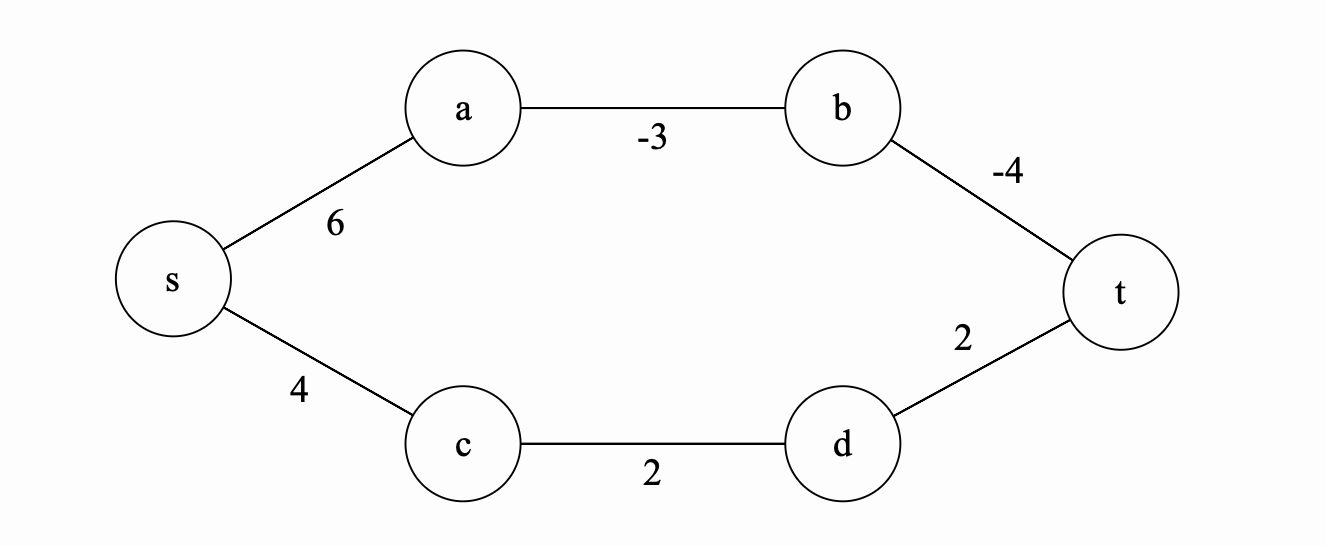
 Consider the graph above and let’s assume that we already know all the shortest paths using at most 2 edges from \(s\) to any vertex in \(G\). So for example, we know that \(D[a,2]=6\), \(D[b,2]=8\), \(D[c,2]=4\) and \(D[t,2]=7\). So now we know the shortest distance from \(s\) to \(t\) using at most two edges is 7. Can we get a shorter path by considering any path that uses 3 edges? Yes!!! we can use the shortest path from \(s\) to \(b\) instead of length 8 and then take in \((b,t)=-4\) to get a shorter path of length 4. In other words, forget about the path \(s->c->t\) and go through \(s->a->b->t\). How can we put this together formally?
Given a vertex \(v \in V\). To find \(D[v,i+1]\), we need to see if for any vertex \(u \in V\), the length of the shortest path from \(s\) to \(u\) using at most \(i\) edges (in other words \(D[u, i]\)) plus \(w(u,v)\) has a lower value than we currently have in \(D[v,i]\). More formally,
With the base case that for \(i = 0\), \(D[s,0]=0\) and \(D[v,0]=\infty\) for all \(v \in V-\{s\}\).
Bellman-Ford and Dijkstra
So what is the relationship between Bellman-Ford and Dijkstra? are they connected in any way? Let’s think about this. We know that in every iteration of Dijkstra’s algorithm, we pick the node with the smallest estimate and then check all the immediate neighbors to see whether any of the neighbors distances’ can be updated. Dijkstra smartly picks the right vertex in every iteration. However, in Bellman-Ford, we just check all of vertices every single iteration. So it’s slower, but now we can find the shortest paths in graphs with negative edges.
Implementation
void BellmanFord(graph& g) {
	int distance[g.size()], parent[g.size()];
	for (int i = 0; i < g.size(); i++) {
	    distance[i] = INT_MAX;
	    parent[i] = -1; // if we need to recover the path
	}
	distance[0] = 0; // source is node 1
	for (int s = 1; s <= g.size() - 1; s++) { // for every possible path size
	    // for every edge in the graph // double loop
	    for (int i = 0; i < g.size(); i++) {
	        for (auto e = g[i].begin(); e != g[i].end(); e++) {
	            int y = e->first;
	            int weight = e->second;
	            // Update if we can get from s to i faster
	            if (distance[i] != INT_MAX && distance[i] + weight < distance[y]) {
	                distance[y] = distance[i] + weight;
	            }
	        }
	    }
	}
}
Example
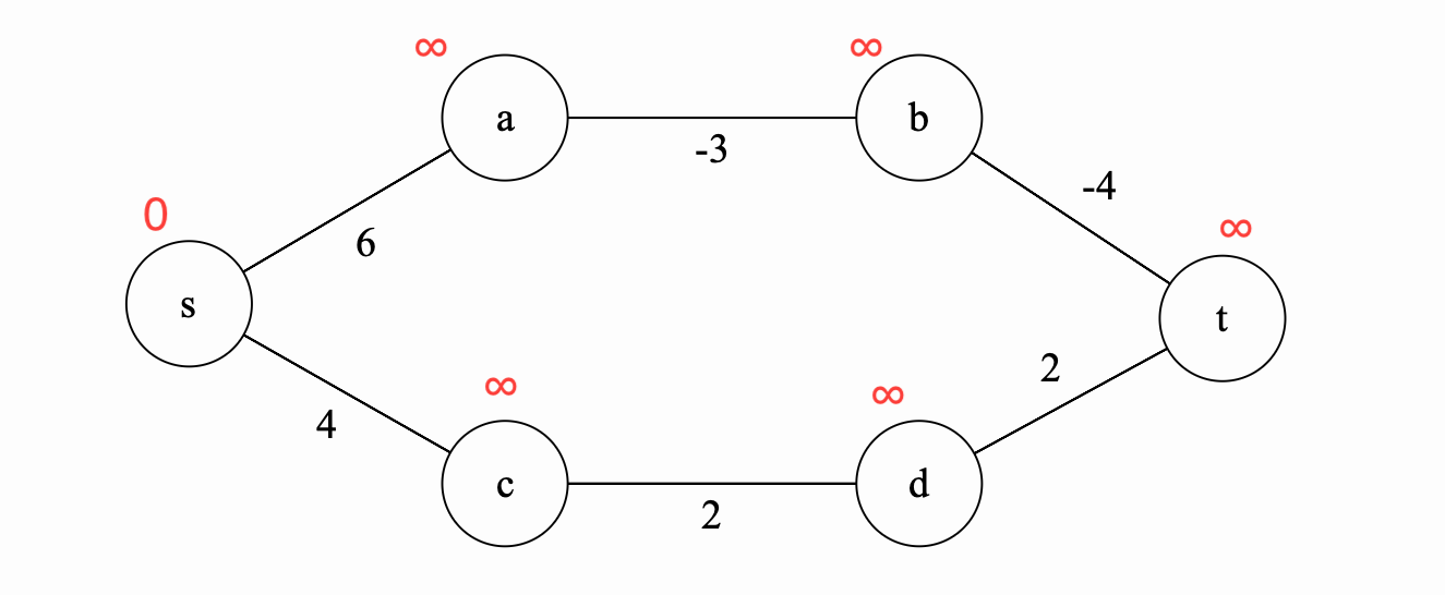
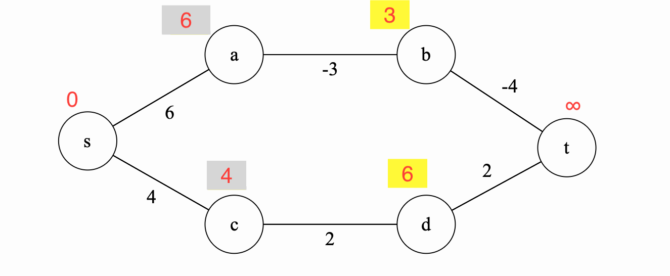
We update according the base case all the shortest paths that use 0 edges to \(\infty\) except for the source vertex where the shortest path is of length 0.
Iteration 1
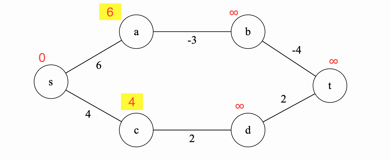
Here we consider the shortest paths using at most 1 edge. We go through every possible \(v \in V\) and every possible neighbor \(u \in v.neighbors\) and ask: Can \(D[v, 1]\) be lowered via the shortest path \(D[u, 0]\) plus the edge \(\{u,v\}\)? The answer is yes! picture below:
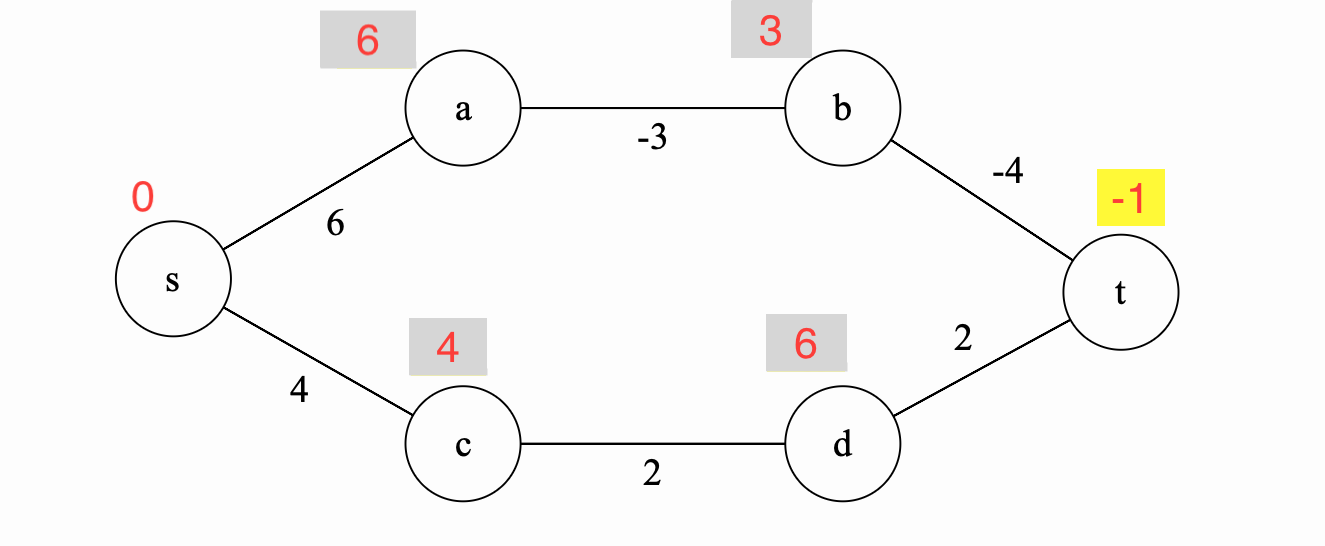
Iteration 2
We repeat the same process, this time we see if we can update all shortest paths that use at most \(2\) edges to better estimates. Notice that we update both \(b\) and \(d\) in this iteration.
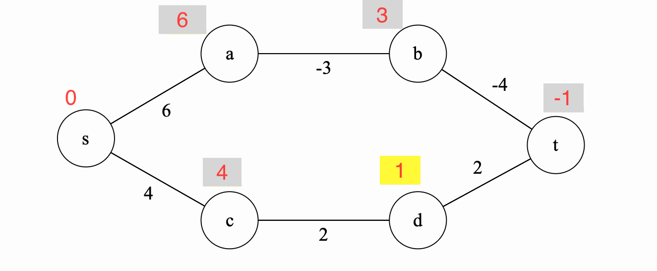
Iteration 3
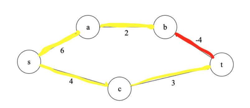
We again repeat the same process, updating this time \(t\).
Iteration 4
In iteration 4, we update \(d\) again because we realize that we can get a better estimate coming through \(t\) instead of \(c\).
Iteration 5
Finally, we update \(c\) because it has a better update now coming through \(d\) instead of directly through \(s\).
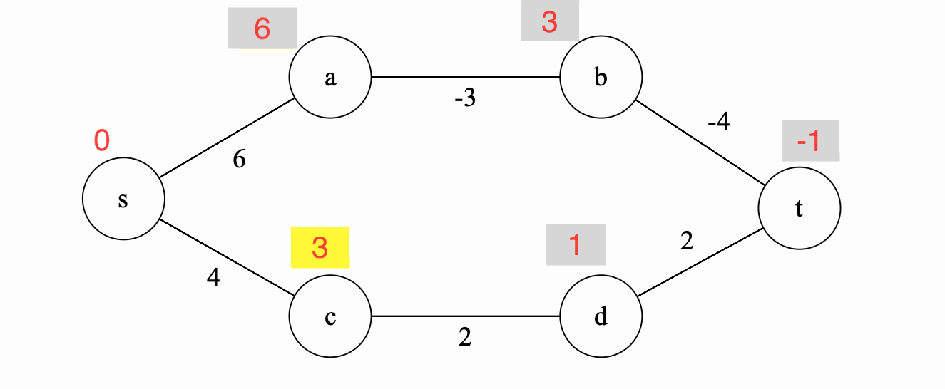 As this point, the algorithm terminates and we have the final shortest paths from \(s\) to every vertex \(v \in V\).
Can we have negative cycles?
If \(G\) has negative cycles then the shortest paths are not defined. They are not defined because you can always find a shorter path by traversing the negative cycle one more time. Bellman-Ford could however detect negative cycles by just doing another iteration and checking if the lengths are continuing to decrease. If they decrease, then we know we have a cycle and we can exit and report that. The sample code below can be added to the above implementation before returning from the function:
We can add one additional iteration to discover negative cycles:
for (int i = 0; i < g.size(); i++) { // for every edge in the graph
    for (auto e = g[i].begin(); e != g[i].end(); e++) {
        int y = e->first;
        int weight = e->second;
        if (distance[i] != INT_MAX && distance[i] + weight < distance[y]) {
            printf("negative weight cycle\n");
        }
    }
}
Why only \(n-1\) iterations?
To answer this question, we ask: can we have positive cycles in a shortest path? The answer is again no. Suppose that we are given a shortest path with a positive weight cycle. Then we can remove the cycle from the path and arrive at a shorter path. This is a contradiction and therefore, we can not have positive weight cycles. Additionally if the cycle is of zero weight or length, then removing the cycle from the shortest path will produce a path with the same weight/length. Therefore, we can restrict finding the shortest path problem to finding a simple shortest path. Simple paths in a graph with \(n\) vertices can have at most \(n-1\) edges and therefore, all we need to do is run Bellman-Ford for \(n-1\) iterations. (CLRS page 645)
Correctness Proof
| Theorem: Given a graph \(G=(V,E)\) and a source vertex \(s\), Bellman-Ford correctly finds the shortest simple paths from \(s\) to every other node in \(G\) |
Proof:
Inductive Hypothesis: After ith iteration, for every \(v \in V\), \(D[v, i]\) is length of the shortest simple path from \(s\) to \(v\) with at most \(i\) edges.
Base Case: After 0th iteration, we have \(D[s, 0] = 0\) and \(D[v, 0]=\infty\) for any \(v \in V - \{s\}\) as required.
Inductive Step: Suppose the inductive hypothesis holds for \(i\). We want to prove it for \(i+1\). Let \(v\) be a vertex in \(V\). Assume there exists a shortest path between \(s\) and \(v\). Let \(u\) be the vertex right before \(v\) on this path. By the inductive hypothesis, we know that \(D[u, i]\) is the length of the shortest simple path between \(s\) and \(u\). In the \(i+1\)‘st iteration, we ensure that we have \(D[v, i+1] \leq D[u, i]+w(u,v)\) by the relaxation step and we also know that \(D[v, i+1]\) is greater or equal than the length of the shortest path from \(s\) to \(v\) with at most \(i+1\) (Are we saying \(D[v,i+1]\) is an overestimate? don’t we have to prove it like Dijkstra?). Therefore, \(D[v, i+1]\) is the length of the shortest path between \(s\) and \(v\) of at most \(i+1\) edges.
Conclusion: After \(n-1\) iterations, for every \(v \in V\), \(D[v, n-1]\) is length of the shortest simple path from \(s\) to \(v\) with at most \(n-1\) edges.
Running Time
Assume we have \(n\) vertices and \(m\) edges. We have \(n-1\) iterations. In each iteration we check every single edge in the graph. Therefore, the running time is \(O(nm)\).