 Let \(G=(V,E)\) be undirected, weighted graph with \(V\) vertices and \(E\) edges. A minimum spanning tree is a tree that connects all the vertices in \(V\) of minimal cost. Prim greedily finds the minimum spanning tree by growing a tree. We start from a vertex and then we pick the cheapest edge out of that vertex. We keep adding cheap edges such that we don’t create a cycle until we cover all the vertices in \(V\). Even though we will only analyze the efficient implementation of Prim, it is very useful to look at the naive implementation because it is more intuitive.
Algorithm
We can start from any node s.
pick the lightest node coming out of s.
MST = [{s,u}]
visited = {s,u}
while |visited| < |V| {
	pick the cheapest edge {x,y} in E so that:
		x is in visited
		y is not in visited
	add {x,y} to MST
	add y to visited
}
return MST
Algorithm (fast, used for the remaining of these notes)
This smart implementation is basically Dijkstra! The only difference is the update condition. In Dijkstra, we take into account the whole path cost while in Prim we only care about the edge weight itself!
Set all vertices to unreached
k[v] = infinity for all v in V
p[u] = -1 for all v in V
k[s] = 0
while there are unreached nodes {
	pick the unreached node u with the smallest key k[u].
	for each neighbor v of u {
		if (k[v] < weight(u,v)) {
			// The is the only difference between Prim and Dijkstra
			k[v] = weight(u,v)
			p[v] = u
		}
	}
	Mark u as reached and add (p[u],u) to MST
	// This edge is safe to add and won't rule out success, proof below!
	// in the actual implementation, we don't add the source vertex since p[u] is -1!
}
Example
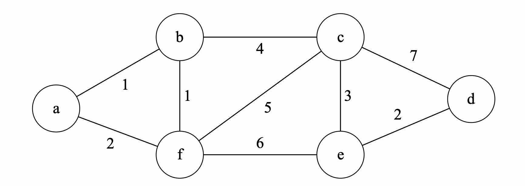
very similar to Dijkstra, we maintain a set of unreached nodes \(\{a, b, c, d, e, f\}\). We then assign \(k[v] = \infty\) for all nodes. For the start node, we update its key to zero. \(k[a] = 0\).
Iteration 0
We extract the minimum unreached node \(a\). We we now update each neighbor according to the algorithm. After updating each neightbor we get the following the values. Also, after updating all neighbors, we mark \(a\) as reached.
| Iteration | a | b | c | d | e | f |
|---|---|---|---|---|---|---|
| 0 (extract \(a\)) | 0 | 1 | \(\infty\) | \(\infty\) | \(\infty\) | 2 |
Iteration 1
We extract the minimum again from the unreached nodes. This time we extract \(b\). We update all the neighbors and at the end of this iteration, we mark \(b\) as sure and \(\{b,a\}\)
| Iteration | a | b | c | d | e | f |
|---|---|---|---|---|---|---|
| 0 (extract \(a\)) | 0 | 1 | \(\infty\) | \(\infty\) | \(\infty\) | 2 |
| 1 (extract \(b\)) add \(\{b,a\}\) | 0 | 1 | 4 | \(\infty\) | \(\infty\) | 1 |
Final iterations
We continue with the same process. We extract the node \(f\) and update its neighbors. We then mark it as reached and add \(\{f,b\}\) to our MST. We next extract \(c\) and update the neighbors again. We then mark \(c\) as reached add \(\{a,b\}\) to our MST. The rest of iterations are in the following table:
| Iteration | a | b | c | d | e | f |
|---|---|---|---|---|---|---|
| 0 (extract \(a\)) | 0 | 1 | \(\infty\) | \(\infty\) | \(\infty\) | 2 |
| 1 (extract \(b\)) add \(\{b,a\}\) | 0 | 1 | 4 | \(\infty\) | \(\infty\) | 1 |
| 2 (extract \(f\)) add \(\{f,b\}\) | 0 | 1 | 4 | \(\infty\) | 6 | 1 |
| 3 (extract \(c\)) add \(\{c,b\}\) | 0 | 1 | 4 | 7 | 3 | 1 |
| 3 (extract \(e\)) add \(\{e,c\}\) | 0 | 1 | 4 | 2 | 3 | 1 |
| 3 (extract \(d\)) add \(\{d,e\}\) | 0 | 1 | 4 | 2 | 3 | 1 |
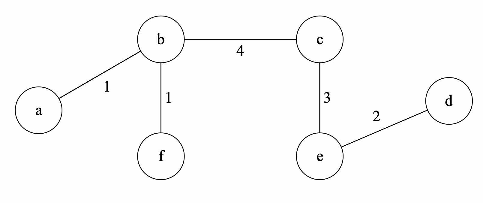
The final minimum spanning tree is the following tree:
Proof of Correctness (Preliminarily)
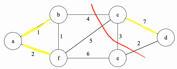
Why does this algorithm find a minimum spanning tree? Before we can answer that, let’s define some terms and prove some lemma that will be useful in the main proof. Let \(G=(V,E)\) be the graph below and let \(S\) be the set of yellow edges in \(G\).
-
A cut is a partition of the vertices into two non-empty disjoint sets. In the graph above, let the vertices on the left of the red line be in \(V_1 = \{a,b,f,e\}\) and let \(V_2 = V - V_1 = \{c,d\}\) be the vertices on the right of the red line.
-
Suppose we have the cut \(\{V_1, V_2 = V - V_1\}\). Define the set of edges that cross the cut to be all edges \(\{u,v\}\) such that \(u \in V_1\) and \(v \in V_2\). Therefore, we will have \(\{(b,c),(c,f),(c,e),(e,d)\}\) in this set.
-
Suppose we have a set of edges \(S\) (highlighted in yellow above). A cut respects \(S\) if no edges in \(S\) cross the cut. None of the yellow edges cross the cut \(\{V_1, V_2\}\).
-
An edge crossing the cut is called light if it has the smallest weight of any edge crossing the cut. In this case, \(\{e,d\}\) is a light edge.
| Lemma: Let \(S\) be a set of edges and consider a cut that respects \(S\). Suppose there is an MST containing \(S\). Let \(\{u,v\}\) be a light edge. Then there is an MST containing \(S \cup \{u,v\}\) |
Proof: Let \(S\) be a set of edges and and consider a cut that respects \(S\). Let \(T\) be an MST containing \(S\). Let \(\{u,v\}\) be a light edge. There are two cases.
Case 1: \(\{u,v\}\) is in \(T\), then we’re done.
Case 2: \(\{u,v\}\) is not in \(T\). By the definition of MST, adding \(\{u,v\}\) will create a cycle in \(T\). Since the sets resulting from the cut must be non-empty. This means that we must have an edge that crosses the cut in \(T\). Let that edge be \(\{x,y\}\). Consider replacing \(\{u,v\}\) with \(\{x,y\}\) to produce the new tree \(T'\). \(T\) is still an MST since we deleted \(\{x,y\}\). \(T'\) has also a cost of at most the cost of \(T\) since {u,v} is a light edge. Therefore, \(T'\) is an MST which includes both \(\{u,v\}\) and \(S\) which is what we wanted to show. \(\blacksquare\)
Prim's Proof of Correctness
| Theorem: Prim will correctly find a minimum spanning tree |
Proof:
Inductive Hypothesis: After adding the \(t\)‘th edge, there exists an MST with the edges added so far.
Base Case: After adding the 0’th edge, there exists an MST with the edges added so far.
Inductive Step: Suppose the inductive hypothesis holds for \(t\). Let \(S\) be the set containing the edges added so far and so there is an MST extending them by the inductive hypothesis. Consider the cut \(S\) and \(V-S\). This cut respects \(S\). Prim adds the lightest edge crossing this cut. By the Lemma above that edge is safe to add. Therefore, there is still an MST extending the new set of edges.
Conclusion: After adding the \(n-1\)‘st edge, there exists an MST with the edges added so far. At this point we have reached all vertices and the \(n-1\) edges we have is an MST.\(\blacksquare\)
Running Time
The analysis is exactly like Dijkstra!. What are we doing in this algorithm? For each vertex in the unreached list, we
(1) find the minimum vertex.
(2) remove that vertex.
(3) update all neighbors with lower key values if possible.
Therefore we see that if we have \(n\) vertices and \(m\) edges:
Now it is clear that it really depends on how we implement the list that holds the not-sure nodes. Let’s consider different data structures
- Arrays
- findMin will run in \(O(n)\)
- RemoveMin will run in \(O(n)\)
- UpdateKey will run in \(O(1)\)
Therefore, the total time will be \(O(n(2n) + m) = O(n^2 + m) = O(n^2)\)
- Red Black Tree
- findMin will run in \(O(\log(n))\)
- RemoveMin will run in \(O(\log(n))\)
- UpdateKey will run in \(O(\log(n))\)
Therefore, the total time will be \(O(n\log(n) + m\log(n)) = O((n+m)\log(n))\).
Notice here, if the graph is dense, meaning that \(m=O(n^2)\), then this is worse than arrays! if it’s sparse, then it’s better.
- Fibonacci Heaps
- findMin will run in \(O(1)\), amortized time.
- RemoveMin will run in \(O(\log(n))\), amortized time.
- UpdateKey will run in \(O(1)\), amortized time.
Therefore, the total time will be \(O(n\log(n) + m)\), amortized time.
Implementation
References
- CS161 @ Stanford with Mary Wootters
- CLRS