Overview
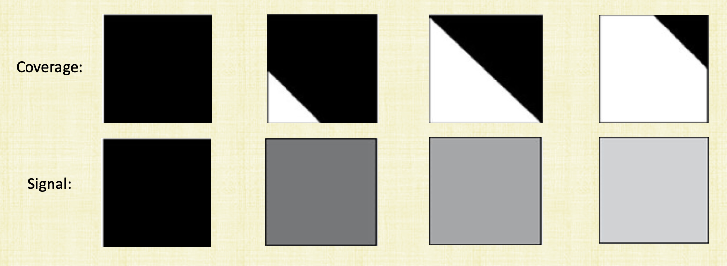
See the above figure. The sensor (which mimics the eye) gets a signal based on how much area is covered by an object. For the first black square we have full coverage and the object is covering the entire sensor and so we get a black signal. The third square is half covered and we’ll get a gray signal. Basically, the sensor averages the information it gets and sends a single based on that. However when perform ray tracing and send a ray out, we’re only sending a ray from the center of the pixel. So for the last square for example, we’re going to see white only instead of some shade of gray and hence we’re losing some information.
Aliasing
Sampling is just testing a single point by sending a ray from the center of the pixel only. Aliasing on the other hand is caused by sampling. Anti-Aliasing is then the solution to aliasing and that’s our goal.
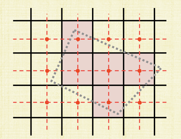
For example, see the above figure. We’re trying to draw a quadrilateral so we send a single ray from each pixel’s center. Do our intersection test with the geometry and find out the centers that do intersect. We color these pixels and end up with a shape that’s completely different (purple squares). Testing the center of the pixel only therefore causes jagged edges often called jaggies. Aliasing can also occur not just with rasterization but also when computing the normal vectors since w’re not computing every single normal which could cause erroneous sparking highlights. Other artifacts causing by sampling include the wagon wheel effect, moire and many more.
Super Sampling
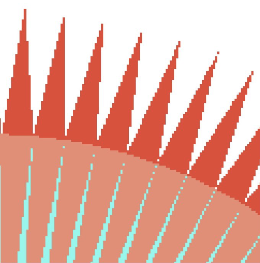
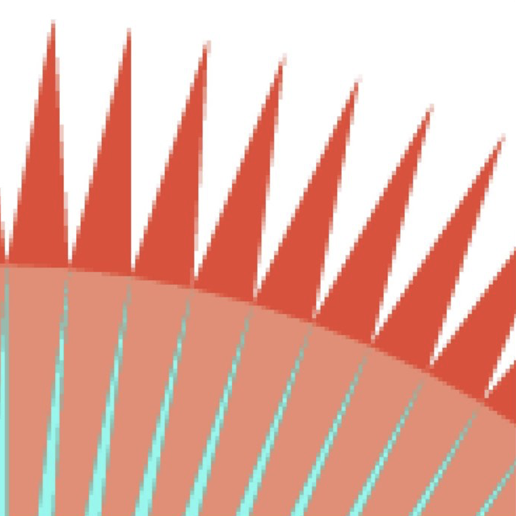
One solution to the aliasing issue is to increase the number of samples (per unit area). We can do this by increasing the number of pixels in the image but now we’ll take longer to render and the file will be much bigger. So far, we’ve used one sample per pixel but now we’ll take 2x2 samples per pixel and then average the result and save that instead for the pixel. This is what super sampling mean. And so instead of Jaggies, we’ll see this
Sampling Rate
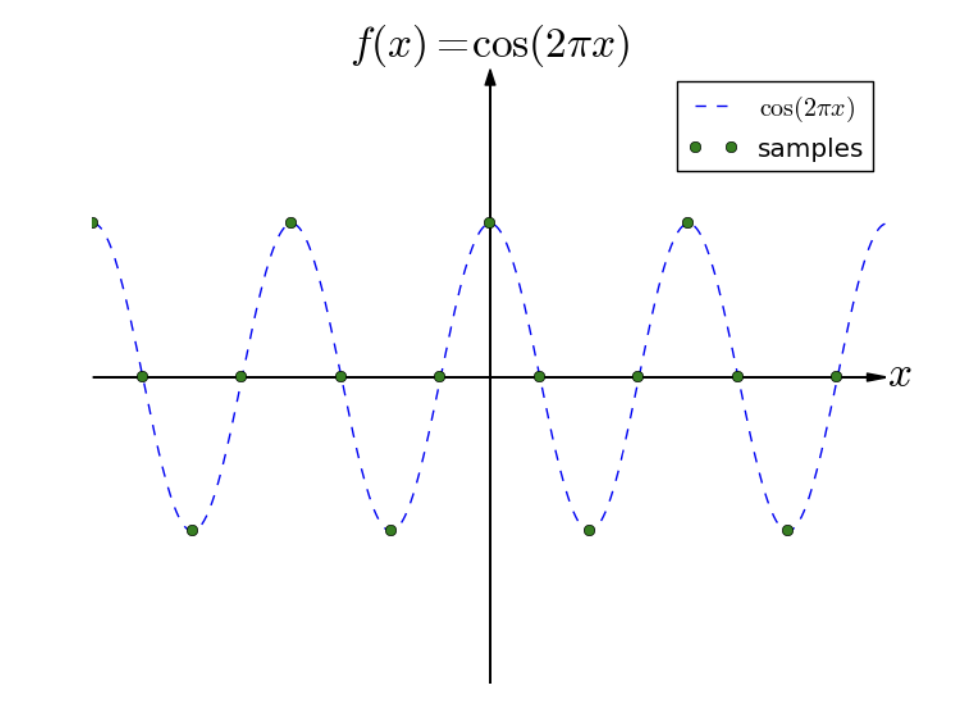
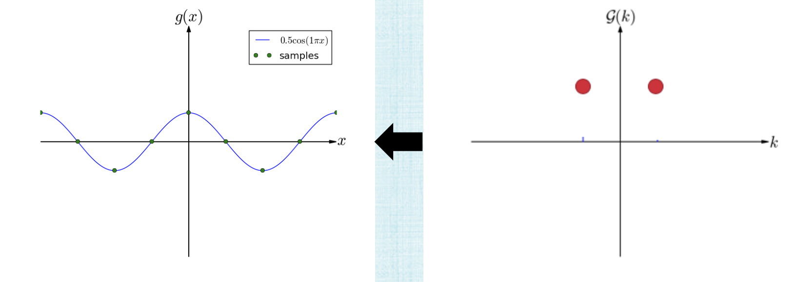
Supersampling is great but what we really want to do in general is to find the lowest possible sampling rate that will not result in noticeable artifacts. Take the cosine function example. See below that whether we chose 4 samples or 2 samples per period, we still don’t lose any information when we reconstruct it from the samples we took.

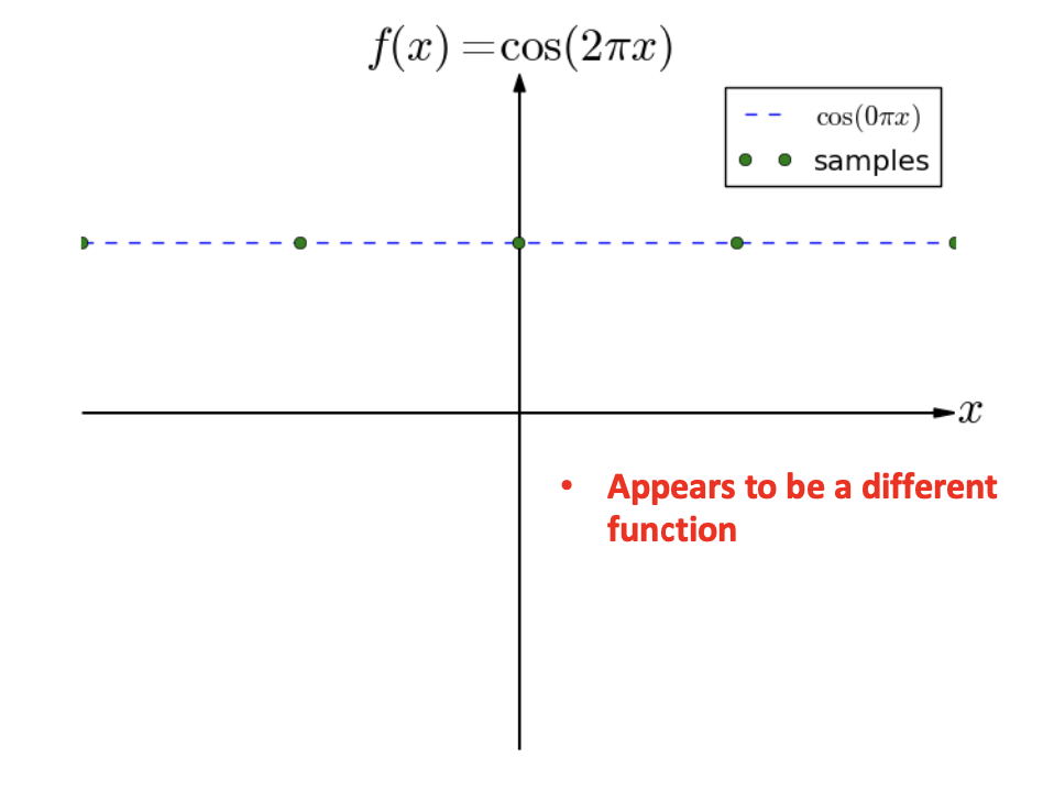
However, if our sample rate was only 1, then we see that we’ve lost information and so it appears that we would need 2 samples ata minimum.
Anti Aliasing
-
Nyquist-Shannon Sampling Theorem says that if $f(t)$ contains no frequencies higher than $W$ hertz, it can be completely determined by samples spaced $1/2W$ seconds apart. So we need 2 samples per period.
-
The Nyquist frequency is defined as half the sampling frequency. If the function being sampled has no frequencies above the Nyquist frequency, then no aliasing occurs.
-
Real world frequencies above the Nyquist frequency appears as aliases to the sampler.
-
Before sampling, remove frequencies higher than the Nyquist frequency.
It needs to be before sampling, otherwise these higher frequencies will get reconstructed as low frequency and get mixed with the real low frequency waves and so we won’t be to differentiate between the two. To remove these frequencies, we use the Fourier Transform.
Fourier Transform
Transforms between the spatial domain $f(x)$ and the frequency domain $F(k)$. Frequency Domain $F(x)$:
Spatial Domain $f(x)$:
where
and
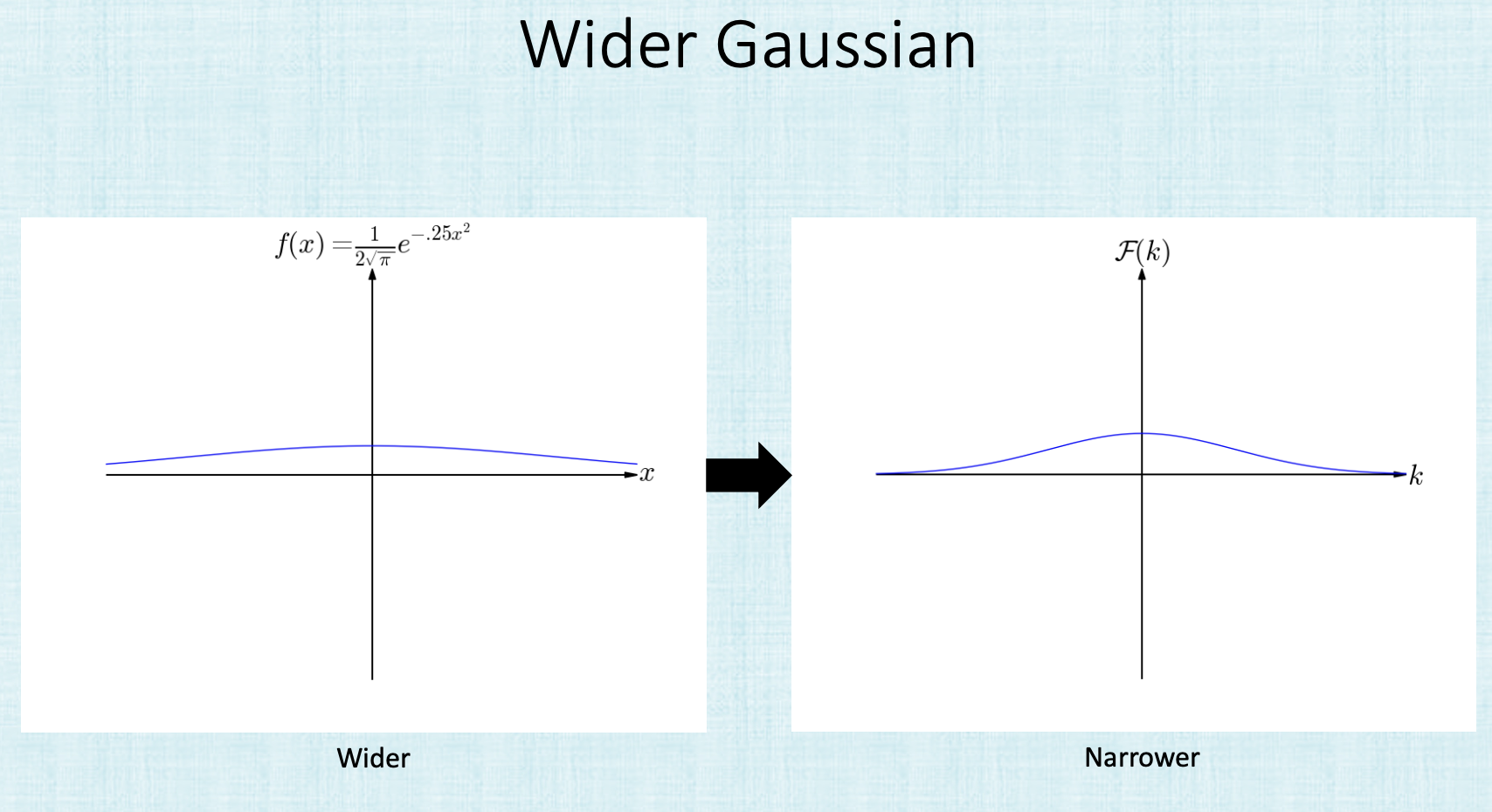
Examples of functions and their Fourier transform below
Anti-Aliasing
Suppose we have this function with $F(k)$,
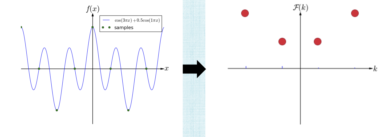
So we first have to identify the nyquist bounds
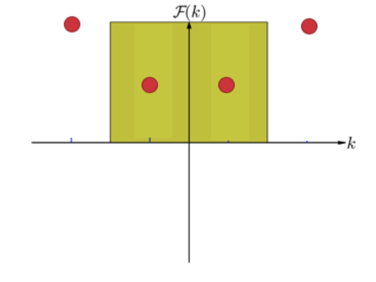
and then remove them (low pass filter) and find the inverse of the Fourier transform
the summary of this process is: Sampling causes higher frequencies to masquerade as lower frequencies and so after sampling, we can no longer untangle the high/low frequencies. So remove these high frequencies to avoid aliasing. Part of the signal will be lost but that’s unavoidable anyways.
This is an example of what happens after removing the high frequencies:

Images
Images have discrete values unlike continuos functions and so we need to use discrete Fourier transform. The Fast Fourier Transform (FFT) computes the discrete Fourier transform and its inverse in $O(nlogn)$ where $n$ is the number of samples. Since images are 2D, we need a 2D discrete transform using 1D transforms after each dimension. Two Example:
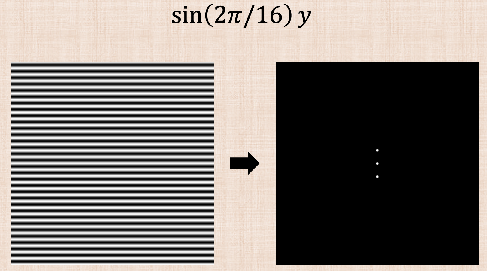
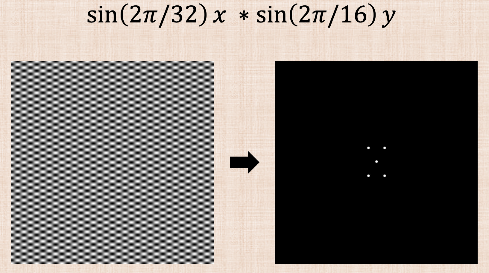
More interesting examples in the slides!
The Pat’s examples shows how edges in images have the highest frequencies! which makes sense since this is where we have the jagged lines.
Convolution
So now we have all the geometry in the scene. We need to get rid of the high frequencies before running the ray tracer or before projecting into screen space!! sending rays from the pixel center is sampling so we need to do this before to avoid getting the high and low frequencies mixed (or high frequencies masquerading as low frequencies). So what we need is to first find a way to run a Fourier transform on the world. hmmm (the world is not a function or an image) …. We can’t do this but what we can do is apply a convolution … A convolution is a way to get the same answer as if we went into the frequency domain.
Let $f$ and $g$ be functions in the spatial domain (e.g. images). When we push $f$ and $g$ into the frequency domain, we’ll call them $F(f)$ and $F(g)$ (transformations of $f$ and $g$ into the frequency domain). In the previous example, $f$ was the image (left) and $F(f)$ was the frequency domain version (right).
Running a low pass filter or removing high frequencies of $F(f)$ is done by multiplying by a Heaviside function $F(g)$ where it’s 1 for low frequencies and 0 for higher frequencies.. The inverse transform will then be $F^{-1}(F(f)F(g))$.
References
Fundamentals of Computer Graphics, 4th Edition
CS148 Lectures
Computer Graphics by Kayvon Fatahalian